Backends#
SAX Backends
import jax
import jax.numpy as jnp
import klujax
import networkx as nx
import sax
Introduction#
SAX allows to easily interchange the backend of a circuit. A SAX backend consists of two static analysis steps and an evaluation step:
- analyze_instances(instances, models)[source]#
- Parameters:
instances (Dict[str, Component]) –
models (Dict[str, Model]) –
- Return type:
Any
- analyze_circuit(analyzed_instances, connections, ports)[source]#
- Parameters:
analyzed_instances (Any) –
connections (Dict[str, str]) –
ports (Dict[str, str]) –
- Return type:
Any
- evaluate_circuit(analyzed, instances)[source]#
- Parameters:
analyzed (Any) –
instances (Dict[str, SType]) –
- Return type:
SType
The analyze_instances step analyzes the ‘shape’ of the instances by running each model with default parameters. By shape we mean which port-combinations are present in the sparse S-matrix.
Warning
QUESTION: can we do this more efficiently in a functional way?
After analyzing the instances, it is assumed that the shape of the instance won’t change any more. It is therefore important that you write your model functions in such a way that the port combinations present in your s-matrix never changes!
Note
we used to do this analysis step in analyze_circuit by just looking at the connections present. However, this inherently assumed dense connectivity within the model. This is pretty inefficient for large sparse models with many ports. Ideally, however, we should be able to analyze the shape of our instances without running their models with default parameters…
The analyze_circuit step should statically analyze the connections and ports and should return an analyzed object. This object contains all the static objects that are needed for circuit computation but won’t be recalculated when any parameters of the circuit change. See KLU Backend (below) for a non-trivial implementation of the circuit analyzation.
The evaluate_circuit step evaluates the circuit for given SType instances, given whatever analysis object was returned from the analyze_circuit step and the instance STypes.
Example#
wg_sdict: sax.SDict = {
    ("in0", "out0"): 0.5 + 0.86603j,
    ("out0", "in0"): 0.5 + 0.86603j,
}

τ, κ = 0.5**0.5, 1j * 0.5**0.5
dc_sdense: sax.SDense = (
    jnp.array([[0, 0, τ, κ], [0, 0, κ, τ], [τ, κ, 0, 0], [κ, τ, 0, 0]]),
    {"in0": 0, "in1": 1, "out0": 2, "out1": 3},
)

instances = {
    "dc1": {"component": "dc"},
    "wg": {"component": "wg"},
    "dc2": {"component": "dc"},
}
connections = {
    "dc1,out0": "wg,in0",
    "wg,out0": "dc2,in0",
    "dc1,out1": "dc2,in1",
}
ports = {
    "in0": "dc1,in0",
    "in1": "dc1,in1",
    "out0": "dc2,out0",
    "out1": "dc2,out1",
}
models = {
    "wg": lambda: wg_sdict,
    "dc": lambda: dc_sdense,
}

analyzed_instances = sax.backends.analyze_instances(instances, models)
analyzed_circuit = sax.backends.analyze_circuit(analyzed_instances, connections, ports)
mzi_sdict = sax.sdict(
    sax.backends.evaluate_circuit(
        analyzed_circuit, {k: models[v["component"]]() for k, v in instances.items()}
    )
)
mzi_sdict
{('in0', 'in0'): Array(0.+0.j, dtype=complex128),
 ('in0', 'in1'): Array(0.+0.j, dtype=complex128),
 ('in0', 'out0'): Array(-0.25+0.433015j, dtype=complex128),
 ('in0', 'out1'): Array(-0.433015+0.75j, dtype=complex128),
 ('in1', 'in0'): Array(0.+0.j, dtype=complex128),
 ('in1', 'in1'): Array(0.+0.j, dtype=complex128),
 ('in1', 'out0'): Array(-0.433015+0.75j, dtype=complex128),
 ('in1', 'out1'): Array(0.25-0.433015j, dtype=complex128),
 ('out0', 'in0'): Array(-0.25+0.433015j, dtype=complex128),
 ('out0', 'in1'): Array(-0.433015+0.75j, dtype=complex128),
 ('out0', 'out0'): Array(0.+0.j, dtype=complex128),
 ('out0', 'out1'): Array(0.+0.j, dtype=complex128),
 ('out1', 'in0'): Array(-0.433015+0.75j, dtype=complex128),
 ('out1', 'in1'): Array(0.25-0.433015j, dtype=complex128),
 ('out1', 'out0'): Array(0.+0.j, dtype=complex128),
 ('out1', 'out1'): Array(0.+0.j, dtype=complex128)}
Filipsson-Gunnar Backend#
Note
Since The KLU Backend (see below) is Superior to the Filipsson-Gunnar backend, SAX will default (since v0.10.0) to the KLU backend if klujax is installed.name1
The Filipsson-Gunnar backend is based on the following paper:
Filipsson, Gunnar. “A new general computer algorithm for S-matrix calculation of interconnected multiports.” 11th European Microwave Conference. IEEE, 1981.
- analyze_circuit_fg(analyzed_instances, connections, ports)[source]#
- Parameters:
analyzed_instances (Dict[str, SDict]) –
connections (Dict[str, str]) –
ports (Dict[str, str]) –
- Return type:
Any
- evaluate_circuit_fg(analyzed, instances)[source]#
evaluate a circuit for the given sdicts.
- Parameters:
analyzed (Any) –
instances (Dict[str, SType]) –
- Return type:
SDict
Algorithm Walkthrough#
Note
This algorithm gets pretty slow for large circuits. Since SAX v0.10.0 we will default to the superior KLU backend as the KLU backend is now also jittable.
Let’s walk through all the steps of this algorithm. We’ll do this for a simple MZI circuit, given by two directional couplers characterised by dc_sdense with a phase shifting waveguide in between wg_sdict:
instances = {
    "dc1": dc_sdense,
    "wg": wg_sdict,
    "dc2": dc_sdense,
}
connections = {
    "dc1,out0": "wg,in0",
    "wg,out0": "dc2,in0",
    "dc1,out1": "dc2,in1",
}
ports = {
    "in0": "dc1,in0",
    "in1": "dc1,in1",
    "out0": "dc2,out0",
    "out1": "dc2,out1",
}
as a first step, we construct the reversed_ports, it’s actually easier to work with reversed_ports (we chose the opposite convention in the netlist definition to adhere to the GDSFactory netlist convention):
reversed_ports = {v: k for k, v in ports.items()}
The first real step of the algorithm is to create the ‘block diagonal sdict`:
block_diag = {}
for name, S in instances.items():
    block_diag.update(
        {(f"{name},{p1}", f"{name},{p2}"): v for (p1, p2), v in sax.sdict(S).items()}
    )
we can optionally filter out zeros from the resulting block_diag representation. Just note that this will make the resuling function unjittable (the resulting ‘shape’ (i.e. keys) of the dictionary would depend on the data itself, which is not allowed in JAX jit). We’re doing it here to avoid printing zeros but internally this is not done by default.
block_diag = {k: v for k, v in block_diag.items() if jnp.abs(v) > 1e-10}
print(len(block_diag))
block_diag
18
{('dc1,in0', 'dc1,out0'): Array(0.70710678+0.j, dtype=complex128),
 ('dc1,in0', 'dc1,out1'): Array(0.+0.70710678j, dtype=complex128),
 ('dc1,in1', 'dc1,out0'): Array(0.+0.70710678j, dtype=complex128),
 ('dc1,in1', 'dc1,out1'): Array(0.70710678+0.j, dtype=complex128),
 ('dc1,out0', 'dc1,in0'): Array(0.70710678+0.j, dtype=complex128),
 ('dc1,out0', 'dc1,in1'): Array(0.+0.70710678j, dtype=complex128),
 ('dc1,out1', 'dc1,in0'): Array(0.+0.70710678j, dtype=complex128),
 ('dc1,out1', 'dc1,in1'): Array(0.70710678+0.j, dtype=complex128),
 ('wg,in0', 'wg,out0'): (0.5+0.86603j),
 ('wg,out0', 'wg,in0'): (0.5+0.86603j),
 ('dc2,in0', 'dc2,out0'): Array(0.70710678+0.j, dtype=complex128),
 ('dc2,in0', 'dc2,out1'): Array(0.+0.70710678j, dtype=complex128),
 ('dc2,in1', 'dc2,out0'): Array(0.+0.70710678j, dtype=complex128),
 ('dc2,in1', 'dc2,out1'): Array(0.70710678+0.j, dtype=complex128),
 ('dc2,out0', 'dc2,in0'): Array(0.70710678+0.j, dtype=complex128),
 ('dc2,out0', 'dc2,in1'): Array(0.+0.70710678j, dtype=complex128),
 ('dc2,out1', 'dc2,in0'): Array(0.+0.70710678j, dtype=complex128),
 ('dc2,out1', 'dc2,in1'): Array(0.70710678+0.j, dtype=complex128)}
next, we sort the connections such that similar components are grouped together:
from sax.backends.filipsson_gunnar import _connections_sort_key

sorted_connections = sorted(connections.items(), key=_connections_sort_key)
sorted_connections
[('dc1,out1', 'dc2,in1'), ('dc1,out0', 'wg,in0'), ('wg,out0', 'dc2,in0')]
Now we iterate over the sorted connections and connect components as they come in. Connected components take over the name of the first component in the connection, but we keep a set of components belonging to that key in all_connected_instances.
This is how this all_connected_instances dictionary looks initially.
all_connected_instances = {k: {k} for k in instances}
all_connected_instances
{'dc1': {'dc1'}, 'wg': {'wg'}, 'dc2': {'dc2'}}
Normally we would loop over every connection in sorted_connections now, but let’s just go through it once at first:
# for k, l in sorted_connections:
k, l = sorted_connections[0]
k, l
('dc1,out1', 'dc2,in1')
k and l are the S-matrix indices we’re trying to connect. Note that in our sparse SDict notation these S-matrix indices are in fact equivalent with the port names ('dc1,out1', 'dc2,in1')!
first we split the connection string into an instance name and a port name (we don’t use the port name yet):
name1, _ = k.split(",")
name2, _ = l.split(",")
We then obtain the new set of connected instances.
connected_instances = all_connected_instances[name1] | all_connected_instances[name2]
connected_instances
{'dc1', 'dc2'}
We then iterate over each of the components in this set and make sure each of the component names in that set maps to that set (yes, I know… confusing). We do this to be able to keep track with which components each of the components in the circuit is currently already connected to.
for name in connected_instances:
    all_connected_instances[name] = connected_instances

all_connected_instances
{'dc1': {'dc1', 'dc2'}, 'wg': {'wg'}, 'dc2': {'dc1', 'dc2'}}
now we need to obtain all the ports of the currently connected instances.
current_ports = tuple(
    p
    for instance in connected_instances
    for p in set([p for p, _ in block_diag] + [p for _, p in block_diag])
    if p.startswith(f"{instance},")
)

current_ports
('dc2,in1',
 'dc2,in0',
 'dc2,out0',
 'dc2,out1',
 'dc1,in0',
 'dc1,out0',
 'dc1,out1',
 'dc1,in1')
Now the Gunnar Algorithm is used. Given a (block-diagonal) ‘S-matrix’ block_diag and a ‘connection matrix’ current_ports we can interconnect port k and l as follows:
Note: some creative freedom is used here. In SAX, the matrices we’re talking about are in fact represented by a sparse dictionary (an
SDict), i.e. similar to a COO sparse matrix for which the indices are the port names.
Just as before, we’re filtering the zeros from the sparse representation (remember, internally this is not done by default).
block_diag = {k: v for k, v in block_diag.items() if jnp.abs(v) > 1e-10}
print(len(block_diag))
block_diag
18
{('dc1,in0', 'dc1,out0'): Array(0.70710678+0.j, dtype=complex128),
 ('dc1,in0', 'dc1,out1'): Array(0.+0.70710678j, dtype=complex128),
 ('dc1,in1', 'dc1,out0'): Array(0.+0.70710678j, dtype=complex128),
 ('dc1,in1', 'dc1,out1'): Array(0.70710678+0.j, dtype=complex128),
 ('dc1,out0', 'dc1,in0'): Array(0.70710678+0.j, dtype=complex128),
 ('dc1,out0', 'dc1,in1'): Array(0.+0.70710678j, dtype=complex128),
 ('dc1,out1', 'dc1,in0'): Array(0.+0.70710678j, dtype=complex128),
 ('dc1,out1', 'dc1,in1'): Array(0.70710678+0.j, dtype=complex128),
 ('wg,in0', 'wg,out0'): (0.5+0.86603j),
 ('wg,out0', 'wg,in0'): (0.5+0.86603j),
 ('dc2,in0', 'dc2,out0'): Array(0.70710678+0.j, dtype=complex128),
 ('dc2,in0', 'dc2,out1'): Array(0.+0.70710678j, dtype=complex128),
 ('dc2,in1', 'dc2,out0'): Array(0.+0.70710678j, dtype=complex128),
 ('dc2,in1', 'dc2,out1'): Array(0.70710678+0.j, dtype=complex128),
 ('dc2,out0', 'dc2,in0'): Array(0.70710678+0.j, dtype=complex128),
 ('dc2,out0', 'dc2,in1'): Array(0.+0.70710678j, dtype=complex128),
 ('dc2,out1', 'dc2,in0'): Array(0.+0.70710678j, dtype=complex128),
 ('dc2,out1', 'dc2,in1'): Array(0.70710678+0.j, dtype=complex128)}
This is the resulting block-diagonal matrix after interconnecting two ports (i.e. basically saying that those two ports are the same port). Because these ports are now connected we should actually remove them from the S-matrix representation (they are integrated into the S-parameters of the other connections):
for i, j in list(block_diag.keys()):
    is_connected = i == k or i == l or j == k or j == l
    is_in_output_ports = i in reversed_ports and j in reversed_ports
    if is_connected and not is_in_output_ports:
        del block_diag[i, j]  # we're no longer interested in these port combinations

print(len(block_diag))
block_diag
10
{('dc1,in0', 'dc1,out0'): Array(0.70710678+0.j, dtype=complex128),
 ('dc1,in1', 'dc1,out0'): Array(0.+0.70710678j, dtype=complex128),
 ('dc1,out0', 'dc1,in0'): Array(0.70710678+0.j, dtype=complex128),
 ('dc1,out0', 'dc1,in1'): Array(0.+0.70710678j, dtype=complex128),
 ('wg,in0', 'wg,out0'): (0.5+0.86603j),
 ('wg,out0', 'wg,in0'): (0.5+0.86603j),
 ('dc2,in0', 'dc2,out0'): Array(0.70710678+0.j, dtype=complex128),
 ('dc2,in0', 'dc2,out1'): Array(0.+0.70710678j, dtype=complex128),
 ('dc2,out0', 'dc2,in0'): Array(0.70710678+0.j, dtype=complex128),
 ('dc2,out1', 'dc2,in0'): Array(0.+0.70710678j, dtype=complex128)}
Note that this deletion of values does NOT make this operation un-jittable. The deletion depends on the ports of the dictionary (i.e. on the dictionary ‘shape’), not on the values.
We now basically have to do those steps again for all other connections:
from sax.backends.filipsson_gunnar import _interconnect_ports

# for k, l in sorted_connections:
for k, l in sorted_connections[
    1:
]:  # we just did the first iteration of this loop above...
    name1, _ = k.split(",")
    name2, _ = l.split(",")
    connected_instances = (
        all_connected_instances[name1] | all_connected_instances[name2]
    )
    for name in connected_instances:
        all_connected_instances[name] = connected_instances
    current_ports = tuple(
        p
        for instance in connected_instances
        for p in set([p for p, _ in block_diag] + [p for _, p in block_diag])
        if p.startswith(f"{instance},")
    )
    block_diag.update(_interconnect_ports(block_diag, current_ports, k, l))
    for i, j in list(block_diag.keys()):
        is_connected = i == k or i == l or j == k or j == l
        is_in_output_ports = i in reversed_ports and j in reversed_ports
        if is_connected and not is_in_output_ports:
            del block_diag[
                i, j
            ]  # we're no longer interested in these port combinations
This is the final MZI matrix we’re getting:
block_diag
{('dc2,out0', 'dc2,out0'): Array(0.+0.j, dtype=complex128),
 ('dc2,out0', 'dc2,out1'): Array(0.+0.j, dtype=complex128),
 ('dc2,out0', 'dc1,in0'): Array(0.25+0.433015j, dtype=complex128),
 ('dc2,out0', 'dc1,in1'): Array(-0.433015+0.25j, dtype=complex128),
 ('dc2,out1', 'dc2,out0'): Array(0.+0.j, dtype=complex128),
 ('dc2,out1', 'dc2,out1'): Array(0.+0.j, dtype=complex128),
 ('dc2,out1', 'dc1,in0'): Array(-0.433015+0.25j, dtype=complex128),
 ('dc2,out1', 'dc1,in1'): Array(-0.25-0.433015j, dtype=complex128),
 ('dc1,in0', 'dc2,out0'): Array(0.25+0.433015j, dtype=complex128),
 ('dc1,in0', 'dc2,out1'): Array(-0.433015+0.25j, dtype=complex128),
 ('dc1,in0', 'dc1,in0'): Array(0.+0.j, dtype=complex128),
 ('dc1,in0', 'dc1,in1'): Array(0.+0.j, dtype=complex128),
 ('dc1,in1', 'dc2,out0'): Array(-0.433015+0.25j, dtype=complex128),
 ('dc1,in1', 'dc2,out1'): Array(-0.25-0.433015j, dtype=complex128),
 ('dc1,in1', 'dc1,in0'): Array(0.+0.j, dtype=complex128),
 ('dc1,in1', 'dc1,in1'): Array(0.+0.j, dtype=complex128)}
All that’s left is to rename these internal ports of the format {instance},{port} into output ports of the resulting circuit:
circuit_sdict: sax.SDict = {
    (reversed_ports[i], reversed_ports[j]): v
    for (i, j), v in block_diag.items()
    if i in reversed_ports and j in reversed_ports
}
circuit_sdict
{('out0', 'out0'): Array(0.+0.j, dtype=complex128),
 ('out0', 'out1'): Array(0.+0.j, dtype=complex128),
 ('out0', 'in0'): Array(0.25+0.433015j, dtype=complex128),
 ('out0', 'in1'): Array(-0.433015+0.25j, dtype=complex128),
 ('out1', 'out0'): Array(0.+0.j, dtype=complex128),
 ('out1', 'out1'): Array(0.+0.j, dtype=complex128),
 ('out1', 'in0'): Array(-0.433015+0.25j, dtype=complex128),
 ('out1', 'in1'): Array(-0.25-0.433015j, dtype=complex128),
 ('in0', 'out0'): Array(0.25+0.433015j, dtype=complex128),
 ('in0', 'out1'): Array(-0.433015+0.25j, dtype=complex128),
 ('in0', 'in0'): Array(0.+0.j, dtype=complex128),
 ('in0', 'in1'): Array(0.+0.j, dtype=complex128),
 ('in1', 'out0'): Array(-0.433015+0.25j, dtype=complex128),
 ('in1', 'out1'): Array(-0.25-0.433015j, dtype=complex128),
 ('in1', 'in0'): Array(0.+0.j, dtype=complex128),
 ('in1', 'in1'): Array(0.+0.j, dtype=complex128)}
And that’s it. We evaluated the SDict of the full circuit.
Algorithm Improvements#
The Filipsson-Gunar algorithm is
pretty fast for small circuits 🙂
jittable 🙂
differentiable 🙂
GPU-compatible 🙂
This algorithm is however:
really slow for large circuits 😥
pretty slow to jit the resulting circuit function 😥
pretty slow to differentiate the resulting circuit function 😥
There are probably still plenty of improvements possible for this algorithm:
¿ Network analysis (ft. NetworkX ?) to obtain which ports of the block diagonal representation are relevant to obtain the output connection ?
¿ Smarter ordering of connections to always have the minimum amount of ports in the intermediate block-diagonal representation ?
¿ Using
jax.lax.scanin stead of python native for-loops in_interconnect_ports?¿ … ?
Bottom line is… Do you know how to improve this algorithm or how to implement the above suggestions? Please open a Merge Request!
KLU Backend#
The KLU backend is using klujax, which uses the SuiteSparse C++ libraries for sparse matrix evaluations to evaluate the circuit insanely fast on a CPU. The specific algorith being used in question is the KLU algorithm:
Ekanathan Palamadai Natariajan. “KLU - A high performance sparse linear solver for circuit simulation problems.”
- analyze_circuit_klu(analyzed_instances, connections, ports)[source]#
- Parameters:
analyzed_instances (Dict[str, SCoo]) –
connections (Dict[str, str]) –
ports (Dict[str, str]) –
- Return type:
Any
- evaluate_circuit_klu(analyzed, instances)[source]#
- Parameters:
analyzed (Any) –
instances (Dict[str, SType]) –
- Return type:
SDense
Theoretical Background#
The core of the KLU algorithm is supported by klujax, which internally uses the Suitesparse libraries to solve the sparse system Ax = b, in which A is a sparse matrix.
Now it only comes down to shoehorn our circuit evaluation into a sparse linear system of equations \(Ax=b\) where we need to solve for \(x\) using klujax.
Consider the block diagonal matrix \(S_{bd}\) of all components in the circuit acting on the fields \(x_{in}\) at each of the individual ports of each of the component integrated in \(S^{bd}\). The output fields \(x^{out}\) at each of those ports is then given by:
However, \(S_{bd}\) is not the S-matrix of the circuit as it does not encode any connectivity between the components. Connecting two component ports basically comes down to enforcing equality between the output fields at one port of a component with the input fields at another port of another (or maybe even the same) component. This equality can be enforced by creating an internal connection matrix, connecting all internal ports of the circuit:
We can thus write the following combined equation:
But this is not the complete story… Some component ports will not be interconnected with other ports: they will become the new external ports (or output ports) of the combined circuit. We can include those external ports into the above equation as follows:
Note that \(C_{ext}\) is obviously not a square matrix. Eliminating \(x^{in}\) from the equation above finally yields:
We basically found a representation of the circuit S-matrix:
Obviously, we won’t want to calculate the inverse \((I - C_{int}S_{bd})^{-1}\), which is the inverse of a very sparse matrix (a connection matrix only has a single 1 per line), which very often is not even sparse itself. In stead we’ll use the solve_klu function:
Moreover, \(C_{ext}^TS_{bd}\) is also a sparse matrix, therefore we’ll also need a mul_coo routine:
Sparse Helper Functions#
- solve(Ai, Aj, Ax, b)[source]#
Solve for x in the sparse linear system Ax=b.
- Parameters:
Ai (Array) – [n_nz; int32]: the row indices of the sparse matrix A
Aj (Array) – [n_nz; int32]: the column indices of the sparse matrix A
Ax (Array) – [n_lhs? x n_nz; float64|complex128]: the values of the sparse matrix A
b (Array) – [n_lhs? x n_col x n_rhs?; float64|complex128]: the target vector
- Returns:
the result (x≈A^-1b)
- Return type:
x
- dot(Ai, Aj, Ax, x)[source]#
Multiply a sparse matrix with a vector: Ax=b.
- Parameters:
Ai (Array) – [n_nz; int32]: the row indices of the sparse matrix A
Aj (Array) – [n_nz; int32]: the column indices of the sparse matrix A
Ax (Array) – [n_lhs? x n_nz; float64|complex128]: the values of the sparse matrix A
x (Array) – [n_lhs? x n_col x n_rhs?; float64|complex128]: the vector multiplied by A
- Returns:
the result (b=A@x)
- Return type:
b
klujax.solve solves the sparse system of equations Ax=b for x. Where A is represented by in COO-format as (Ai, Aj, Ax).
Example
Ai = jnp.array([0, 1, 2, 3, 4])
Aj = jnp.array([1, 3, 4, 0, 2])
Ax = jnp.array([5, 6, 1, 1, 2])
b = jnp.array([5, 3, 2, 6, 1])
x = klujax.solve(Ai, Aj, Ax, b)
x
Array([6. , 1. , 0.5, 0.5, 2. ], dtype=float64)
This result is indeed correct:
A = jnp.zeros((5, 5)).at[Ai, Aj].set(Ax)
print(A)
print(A @ x)
[[0. 5. 0. 0. 0.]
 [0. 0. 0. 6. 0.]
 [0. 0. 0. 0. 1.]
 [1. 0. 0. 0. 0.]
 [0. 0. 2. 0. 0.]]
[5. 3. 2. 6. 1.]
However, to use this function effectively, we probably need an extra dimension for Ax. Indeed, we would like to solve this equation for multiple wavelengths (or more general, for multiple circuit configurations) at once. For this we can use jax.vmap to expose klujax.solve to more dimensions for Ax:
solve_klu = jax.vmap(klujax.solve, (None, None, 0, None), 0)
Let’s now redefine Ax and see what it gives:
Ai = jnp.array([0, 1, 2, 3, 4])
Aj = jnp.array([1, 3, 4, 0, 2])
Ax = jnp.array([[5, 6, 1, 1, 2], [5, 4, 3, 2, 1], [1, 2, 3, 4, 5]])
b = jnp.array([5, 3, 2, 6, 1])
x = solve_klu(Ai, Aj, Ax, b)
x
Array([[6.        , 1.        , 0.5       , 0.5       , 2.        ],
       [3.        , 1.        , 1.        , 0.75      , 0.66666667],
       [1.5       , 5.        , 0.2       , 1.5       , 0.66666667]],      dtype=float64)
This result is indeed correct:
A = jnp.zeros((3, 5, 5)).at[:, Ai, Aj].set(Ax)
jnp.einsum("ijk,ik->ij", A, x)
Array([[5., 3., 2., 6., 1.],
       [5., 3., 2., 6., 1.],
       [5., 3., 2., 6., 1.]], dtype=float64)
Additionally, we need a way to multiply a sparse COO-matrix with a dense vector. This can be done with klujax.coo_mul_vec:
However, it’s useful to allow a batch dimension, this time both in Ax and in b:
mul_coo = None
mul_coo = jax.vmap(klujax.dot, (None, None, 0, 0), 0)
Let’s confirm this does the right thing:
result = mul_coo(Ai, Aj, Ax, x)
result
Array([[5., 3., 2., 6., 1.],
       [5., 3., 2., 6., 1.],
       [5., 3., 2., 6., 1.]], dtype=float64)
Example#
wg_sdict: sax.SDict = {
    ("in0", "out0"): 0.5 + 0.86603j,
    ("out0", "in0"): 0.5 + 0.86603j,
}

τ, κ = 0.5**0.5, 1j * 0.5**0.5
dc_sdense: sax.SDense = (
    jnp.array([[0, 0, τ, κ], [0, 0, κ, τ], [τ, κ, 0, 0], [κ, τ, 0, 0]]),
    {"out0": 0, "out1": 1, "in0": 2, "in1": 3},
)

instances = {
    "dc1": {"component": "dc"},
    "wg": {"component": "wg"},
    "dc2": {"component": "dc"},
}
connections = {
    "dc1,out0": "wg,in0",
    "wg,out0": "dc2,in0",
    "dc1,out1": "dc2,in1",
}
ports = {
    "in0": "dc1,in0",
    "in1": "dc1,in1",
    "out0": "dc2,out0",
    "out1": "dc2,out1",
}
models = {
    "wg": lambda: wg_sdict,
    "dc": lambda: dc_sdense,
}


analyzed_instances = sax.backends.analyze_instances_klu(instances, models)
analyzed_circuit = sax.backends.analyze_circuit_klu(
    analyzed_instances, connections, ports
)
S, pm = sax.backends.evaluate_circuit_klu(
    analyzed_circuit, {k: models[v["component"]]() for k, v in instances.items()}
)

print(S)
print(pm)
[[ 0.      +0.j        0.      +0.j       -0.25    +0.433015j
  -0.433015+0.75j    ]
 [ 0.      +0.j        0.      +0.j       -0.433015+0.75j
   0.25    -0.433015j]
 [-0.25    +0.433015j -0.433015+0.75j      0.      +0.j
   0.      +0.j      ]
 [-0.433015+0.75j      0.25    -0.433015j  0.      +0.j
   0.      +0.j      ]]
{'in0': 0, 'in1': 1, 'out0': 2, 'out1': 3}
the KLU backend yields SDense results by default:
mzi_sdense = (S, pm)
mzi_sdense
(Array([[ 0.      +0.j      ,  0.      +0.j      , -0.25    +0.433015j,
         -0.433015+0.75j    ],
        [ 0.      +0.j      ,  0.      +0.j      , -0.433015+0.75j    ,
          0.25    -0.433015j],
        [-0.25    +0.433015j, -0.433015+0.75j    ,  0.      +0.j      ,
          0.      +0.j      ],
        [-0.433015+0.75j    ,  0.25    -0.433015j,  0.      +0.j      ,
          0.      +0.j      ]], dtype=complex128),
 {'in0': 0, 'in1': 1, 'out0': 2, 'out1': 3})
An SDense is returned for perfomance reasons. By returning an SDense by default we prevent any internal SDict -> SDense conversions in deeply hierarchical circuits. It’s however very easy to convert SDense to SDict as a final step. To do this, wrap the result (or the function generating the result) with sdict:
sax.sdict(mzi_sdense)
{('in0', 'in0'): Array(0.+0.j, dtype=complex128),
 ('in0', 'in1'): Array(0.+0.j, dtype=complex128),
 ('in0', 'out0'): Array(-0.25+0.433015j, dtype=complex128),
 ('in0', 'out1'): Array(-0.433015+0.75j, dtype=complex128),
 ('in1', 'in0'): Array(0.+0.j, dtype=complex128),
 ('in1', 'in1'): Array(0.+0.j, dtype=complex128),
 ('in1', 'out0'): Array(-0.433015+0.75j, dtype=complex128),
 ('in1', 'out1'): Array(0.25-0.433015j, dtype=complex128),
 ('out0', 'in0'): Array(-0.25+0.433015j, dtype=complex128),
 ('out0', 'in1'): Array(-0.433015+0.75j, dtype=complex128),
 ('out0', 'out0'): Array(0.+0.j, dtype=complex128),
 ('out0', 'out1'): Array(0.+0.j, dtype=complex128),
 ('out1', 'in0'): Array(-0.433015+0.75j, dtype=complex128),
 ('out1', 'in1'): Array(0.25-0.433015j, dtype=complex128),
 ('out1', 'out0'): Array(0.+0.j, dtype=complex128),
 ('out1', 'out1'): Array(0.+0.j, dtype=complex128)}
Algorithm Walkthrough#
Let’s first enforce \(C^T = C\):
connections = {**connections, **{v: k for k, v in connections.items()}}
connections
{'dc1,out0': 'wg,in0',
 'wg,out0': 'dc2,in0',
 'dc1,out1': 'dc2,in1',
 'wg,in0': 'dc1,out0',
 'dc2,in0': 'wg,out0',
 'dc2,in1': 'dc1,out1'}
We’ll also need the reversed ports:
inverse_ports = {v: k for k, v in ports.items()}
inverse_ports
{'dc1,in0': 'in0', 'dc1,in1': 'in1', 'dc2,out0': 'out0', 'dc2,out1': 'out1'}
An the port indices
port_map = {k: i for i, k in enumerate(ports)}
port_map
{'in0': 0, 'in1': 1, 'out0': 2, 'out1': 3}
Let’s now create the COO-representation of our block diagonal S-matrix \(S_{bd}\):
idx, Si, Sj, Sx, instance_ports = 0, [], [], [], {}
batch_shape = ()
for name, instance in instances.items():
    s = models[instance["component"]]()
    si, sj, sx, ports_map = sax.scoo(s)
    Si.append(si + idx)
    Sj.append(sj + idx)
    Sx.append(sx)
    if len(sx.shape[:-1]) > len(batch_shape):
        batch_shape = sx.shape[:-1]
    instance_ports.update({f"{name},{p}": i + idx for p, i in ports_map.items()})
    idx += len(ports_map)
Si = jnp.concatenate(Si, -1)
Sj = jnp.concatenate(Sj, -1)
Sx = jnp.concatenate(
    [jnp.broadcast_to(sx, (*batch_shape, sx.shape[-1])) for sx in Sx], -1
)

print(Si)
print(Sj)
print(Sx)
[0 0 0 0 1 1 1 1 2 2 2 2 3 3 3 3 4 5 6 6 6 6 7 7 7 7 8 8 8 8 9 9 9 9]
[0 1 2 3 0 1 2 3 0 1 2 3 0 1 2 3 5 4 6 7 8 9 6 7 8 9 6 7 8 9 6 7 8 9]
[0.        +0.j         0.        +0.j         0.70710678+0.j
 0.        +0.70710678j 0.        +0.j         0.        +0.j
 0.        +0.70710678j 0.70710678+0.j         0.70710678+0.j
 0.        +0.70710678j 0.        +0.j         0.        +0.j
 0.        +0.70710678j 0.70710678+0.j         0.        +0.j
 0.        +0.j         0.5       +0.86603j    0.5       +0.86603j
 0.        +0.j         0.        +0.j         0.70710678+0.j
 0.        +0.70710678j 0.        +0.j         0.        +0.j
 0.        +0.70710678j 0.70710678+0.j         0.70710678+0.j
 0.        +0.70710678j 0.        +0.j         0.        +0.j
 0.        +0.70710678j 0.70710678+0.j         0.        +0.j
 0.        +0.j        ]
note that we also kept track of the batch_shape, i.e. the number of independent simulations (usually number of wavelengths). In the example being used here we don’t have a batch dimension (all elements of the SDict are 0D):
batch_shape
()
We’ll also keep track of the number of columns
n_col = idx
n_col
10
And we’ll need to solve the circuit for each output port, i.e. we need to solve n_rhs number of equations:
n_rhs = len(port_map)
n_rhs
4
We can represent the internal connection matrix \(C_{int}\) as a mapping between port indices:
Cmap = {int(instance_ports[k]): int(instance_ports[v]) for k, v in connections.items()}
Cmap
{0: 4, 5: 8, 1: 9, 4: 0, 8: 5, 9: 1}
Therefore, the COO-representation of this connection matrix can be obtained as follows (note that an array of values Cx is not necessary, all non-zero elements in a connection matrix are 1)
Ci = jnp.array(list(Cmap.keys()), dtype=jnp.int32)
Cj = jnp.array(list(Cmap.values()), dtype=jnp.int32)
print(Ci)
print(Cj)
[0 5 1 4 8 9]
[4 8 9 0 5 1]
We can represent the external connection matrix \(C_{ext}\) as a map between internal port indices and external port indices:
Cextmap = {int(instance_ports[k]): int(port_map[v]) for k, v in inverse_ports.items()}
Cextmap
{2: 0, 3: 1, 6: 2, 7: 3}
Just as for the internal matrix we can represent this external connection matrix in COO-format:
Cexti = jnp.stack(list(Cextmap.keys()), 0)
Cextj = jnp.stack(list(Cextmap.values()), 0)
print(Cexti)
print(Cextj)
[2 3 6 7]
[0 1 2 3]
However, we actually need it as a dense representation:
help needed: can we find a way later on to keep this sparse?
Cext = jnp.zeros((n_col, n_rhs), dtype=complex).at[Cexti, Cextj].set(1.0)
Cext
Array([[0.+0.j, 0.+0.j, 0.+0.j, 0.+0.j],
       [0.+0.j, 0.+0.j, 0.+0.j, 0.+0.j],
       [1.+0.j, 0.+0.j, 0.+0.j, 0.+0.j],
       [0.+0.j, 1.+0.j, 0.+0.j, 0.+0.j],
       [0.+0.j, 0.+0.j, 0.+0.j, 0.+0.j],
       [0.+0.j, 0.+0.j, 0.+0.j, 0.+0.j],
       [0.+0.j, 0.+0.j, 1.+0.j, 0.+0.j],
       [0.+0.j, 0.+0.j, 0.+0.j, 1.+0.j],
       [0.+0.j, 0.+0.j, 0.+0.j, 0.+0.j],
       [0.+0.j, 0.+0.j, 0.+0.j, 0.+0.j]], dtype=complex128)
We’ll now calculate the row index CSi of \(C_{int}S_{bd}\) in COO-format:
# TODO: make this block jittable...
Ix = jnp.ones((*batch_shape, n_col))
Ii = Ij = jnp.arange(n_col)
mask = Cj[None, :] == Si[:, None]
CSi = jnp.broadcast_to(Ci[None, :], mask.shape)[mask]
CSi
Array([4, 4, 4, 4, 9, 9, 9, 9, 0, 8, 5, 5, 5, 5, 1, 1, 1, 1], dtype=int32)
CSi: possible jittable alternative? how do we remove the zeros?
CSi_ = jnp.where(Cj[None, :] == Si[:, None], Ci[None, :], 0).sum(1)  # not used
CSi_  # not used
Array([4, 4, 4, 4, 9, 9, 9, 9, 0, 0, 0, 0, 0, 0, 0, 0, 0, 8, 0, 0, 0, 0,
       0, 0, 0, 0, 5, 5, 5, 5, 1, 1, 1, 1], dtype=int64)
The column index CSj of \(C_{int}S_{bd}\) can more easily be obtained:
mask = (Cj[:, None] == Si[None, :]).any(0)
CSj = Sj[mask]
CSj
Array([0, 1, 2, 3, 0, 1, 2, 3, 5, 4, 6, 7, 8, 9, 6, 7, 8, 9], dtype=int64)
Finally, the values CSx of \(C_{int}S_{bd}\) can be obtained as follows:
CSx = Sx[..., mask]
CSx
Array([0.        +0.j        , 0.        +0.j        ,
       0.70710678+0.j        , 0.        +0.70710678j,
       0.        +0.j        , 0.        +0.j        ,
       0.        +0.70710678j, 0.70710678+0.j        ,
       0.5       +0.86603j   , 0.5       +0.86603j   ,
       0.70710678+0.j        , 0.        +0.70710678j,
       0.        +0.j        , 0.        +0.j        ,
       0.        +0.70710678j, 0.70710678+0.j        ,
       0.        +0.j        , 0.        +0.j        ], dtype=complex128)
Now we calculate \(I - C_{int}S_{bd}\) in an uncoalesced way (we might have duplicate indices on the diagonal):
uncoalesced: having duplicate index combinations (i, j) in the representation possibly with different corresponding values. This is usually not a problem as in linear operations these values will end up to be summed, usually the behavior you want:
I_CSi = jnp.concatenate([CSi, Ii], -1)
I_CSj = jnp.concatenate([CSj, Ij], -1)
I_CSx = jnp.concatenate([-CSx, Ix], -1)
print(I_CSi)
print(I_CSj)
print(I_CSx)
[4 4 4 4 9 9 9 9 0 8 5 5 5 5 1 1 1 1 0 1 2 3 4 5 6 7 8 9]
[0 1 2 3 0 1 2 3 5 4 6 7 8 9 6 7 8 9 0 1 2 3 4 5 6 7 8 9]
[-0.        -0.j         -0.        -0.j         -0.70710678-0.j
 -0.        -0.70710678j -0.        -0.j         -0.        -0.j
 -0.        -0.70710678j -0.70710678-0.j         -0.5       -0.86603j
 -0.5       -0.86603j    -0.70710678-0.j         -0.        -0.70710678j
 -0.        -0.j         -0.        -0.j         -0.        -0.70710678j
 -0.70710678-0.j         -0.        -0.j         -0.        -0.j
  1.        +0.j          1.        +0.j          1.        +0.j
  1.        +0.j          1.        +0.j          1.        +0.j
  1.        +0.j          1.        +0.j          1.        +0.j
  1.        +0.j        ]
n_col, n_rhs = Cext.shape
print(n_col, n_rhs)
10 4
The batch shape dimension can generally speaking be anything (in the example here 0D). We need to do the necessary reshapings to make the batch shape 1D:
n_lhs = jnp.prod(jnp.array(batch_shape, dtype=jnp.int32))
print(n_lhs)
1
Sx = Sx.reshape(n_lhs, -1)
Sx.shape
(1, 34)
I_CSx = I_CSx.reshape(n_lhs, -1)
I_CSx.shape
(1, 28)
We’re finally ready to do the most important part of the calculation, which we conveniently leave to klujax and SuiteSparse:
inv_I_CS_Cext = solve_klu(I_CSi, I_CSj, I_CSx, Cext)
one more sparse multiplication:
S_inv_I_CS_Cext = mul_coo(Si, Sj, Sx, inv_I_CS_Cext)
And one more \(C_{ext}\) multiplication which we do by clever indexing:
CextT_S_inv_I_CS_Cext = S_inv_I_CS_Cext[..., Cexti, :][..., :, Cextj]
CextT_S_inv_I_CS_Cext
Array([[[ 0.      +0.j      ,  0.      +0.j      , -0.25    +0.433015j,
         -0.433015+0.75j    ],
        [ 0.      +0.j      ,  0.      +0.j      , -0.433015+0.75j    ,
          0.25    -0.433015j],
        [-0.25    +0.433015j, -0.433015+0.75j    ,  0.      +0.j      ,
          0.      +0.j      ],
        [-0.433015+0.75j    ,  0.25    -0.433015j,  0.      +0.j      ,
          0.      +0.j      ]]], dtype=complex128)
That’s it! We found the S-matrix of the circuit. We just need to reshape the batch dimension back into the matrix:
_, n, _ = CextT_S_inv_I_CS_Cext.shape
S = CextT_S_inv_I_CS_Cext.reshape(*batch_shape, n, n)
S
Array([[ 0.      +0.j      ,  0.      +0.j      , -0.25    +0.433015j,
        -0.433015+0.75j    ],
       [ 0.      +0.j      ,  0.      +0.j      , -0.433015+0.75j    ,
         0.25    -0.433015j],
       [-0.25    +0.433015j, -0.433015+0.75j    ,  0.      +0.j      ,
         0.      +0.j      ],
       [-0.433015+0.75j    ,  0.25    -0.433015j,  0.      +0.j      ,
         0.      +0.j      ]], dtype=complex128)
Oh and to complete the SDense representation we need to specify the port map as well:
port_map
{'in0': 0, 'in1': 1, 'out0': 2, 'out1': 3}
Algorithm Improvements#
This algorithm is
very fast for large circuits 🙂
jittable 🙂
differentiable 🙂
This algorithm is however:
not GPU-compatible 🙂
There are probably still plenty of improvements possible for this algorithm:
¿ make it GPU compatible (requires making suitesparse GPU compatible… probably not gonna happen)?
Note
Since The KLU Backend is Superior to the Filipsson-Gunnar backend, SAX will default (since v0.10.0) to the KLU backend if klujax is installed.name1
Additive Backend#
- analyze_circuit_additive(analyzed_instances, connections, ports)[source]#
- Parameters:
analyzed_instances (Dict[str, SDict]) –
connections (Dict[str, str]) –
ports (Dict[str, str]) –
- Return type:
Any
- evaluate_circuit_additive(analyzed, instances)[source]#
evaluate a circuit for the given sdicts.
- Parameters:
analyzed (Any) –
instances (Dict[str, SDict]) –
- Return type:
SDict
Sometimes we would like to calculate circuit path lengths or time delays within a circuit. We could obviously simulate these things with a time domain simulator, but in many cases a simple additive backend (as opposed to the default multiplicative backend) can suffice.
Example#
Note
in stead of S-parameters the stypes need to contain additive parameters, such as length or time delay.
wg_sdict = {
    ("in0", "out0"): jnp.array(
        [100.0, 200.0, 300.0]
    ),  # assume for now there are three possible paths between these two ports.
    ("out0", "in0"): jnp.array(
        [100.0, 200.0, 300.0]
    ),  # assume for now there are three possible paths between these two ports.
}

dc_sdict = {
    ("in0", "out0"): jnp.array(
        [10.0, 20.0]
    ),  # assume for now there are two possible paths between these two ports.
    ("in0", "out1"): 15.0,
    ("in1", "out0"): 15.0,
    ("in1", "out1"): jnp.array(
        [10.0, 20.0]
    ),  # assume for now there are two possible paths between these two ports.
}

instances = {
    "dc1": {"component": "dc"},
    "wg": {"component": "wg"},
    "dc2": {"component": "dc"},
}
connections = {
    "dc1,out0": "wg,in0",
    "wg,out0": "dc2,in0",
    "dc1,out1": "dc2,in1",
}
ports = {
    "in0": "dc1,in0",
    "in1": "dc1,in1",
    "out0": "dc2,out0",
    "out1": "dc2,out1",
}
models = {
    "wg": lambda: wg_sdict,
    "dc": lambda: dc_sdense,
}
Note
it is recommended to not use an SDense representation for the additive backend. Very often an SDense representation will introduce zeros which will be interpreted as an existing connection with zero length. Conversely, in a sparse representation like SDict or SCoo, non-existing elements will be just that: they will not be present in the internal graph.
edges = sax.backends.additive._graph_edges(
    {k: models[v["component"]]() for k, v in instances.items()}, connections, ports
)
edges
/home/runner/work/sax/sax/.venv/lib/python3.12/site-packages/jax/_src/numpy/lax_numpy.py:5566: ComplexWarning: Casting complex values to real discards the imaginary part
  out_array: Array = lax_internal._convert_element_type(
[(('dc1', 'out0'),
  ('wg', 'in0'),
  {'type': 'C', 'length': Array([0.], dtype=float64)}),
 (('wg', 'out0'),
  ('dc2', 'in0'),
  {'type': 'C', 'length': Array([0.], dtype=float64)}),
 (('dc1', 'out1'),
  ('dc2', 'in1'),
  {'type': 'C', 'length': Array([0.], dtype=float64)}),
 (('wg', 'in0'),
  ('dc1', 'out0'),
  {'type': 'C', 'length': Array([0.], dtype=float64)}),
 (('dc2', 'in0'),
  ('wg', 'out0'),
  {'type': 'C', 'length': Array([0.], dtype=float64)}),
 (('dc2', 'in1'),
  ('dc1', 'out1'),
  {'type': 'C', 'length': Array([0.], dtype=float64)}),
 (('', 'in0'),
  ('dc1', 'in0'),
  {'type': 'C', 'length': Array([0.], dtype=float64)}),
 (('', 'in1'),
  ('dc1', 'in1'),
  {'type': 'C', 'length': Array([0.], dtype=float64)}),
 (('', 'out0'),
  ('dc2', 'out0'),
  {'type': 'C', 'length': Array([0.], dtype=float64)}),
 (('', 'out1'),
  ('dc2', 'out1'),
  {'type': 'C', 'length': Array([0.], dtype=float64)}),
 (('dc1', 'in0'),
  ('', 'in0'),
  {'type': 'C', 'length': Array([0.], dtype=float64)}),
 (('dc1', 'in1'),
  ('', 'in1'),
  {'type': 'C', 'length': Array([0.], dtype=float64)}),
 (('dc2', 'out0'),
  ('', 'out0'),
  {'type': 'C', 'length': Array([0.], dtype=float64)}),
 (('dc2', 'out1'),
  ('', 'out1'),
  {'type': 'C', 'length': Array([0.], dtype=float64)}),
 (('dc1', 'out0'),
  ('dc1', 'out0'),
  {'type': 'S', 'length': Array([0.], dtype=float64)}),
 (('dc1', 'out0'),
  ('dc1', 'out1'),
  {'type': 'S', 'length': Array([0.], dtype=float64)}),
 (('dc1', 'out0'),
  ('dc1', 'in0'),
  {'type': 'S', 'length': Array([0.70710678], dtype=float64)}),
 (('dc1', 'out0'),
  ('dc1', 'in1'),
  {'type': 'S', 'length': Array([0.], dtype=float64)}),
 (('dc1', 'out1'),
  ('dc1', 'out0'),
  {'type': 'S', 'length': Array([0.], dtype=float64)}),
 (('dc1', 'out1'),
  ('dc1', 'out1'),
  {'type': 'S', 'length': Array([0.], dtype=float64)}),
 (('dc1', 'out1'),
  ('dc1', 'in0'),
  {'type': 'S', 'length': Array([0.], dtype=float64)}),
 (('dc1', 'out1'),
  ('dc1', 'in1'),
  {'type': 'S', 'length': Array([0.70710678], dtype=float64)}),
 (('dc1', 'in0'),
  ('dc1', 'out0'),
  {'type': 'S', 'length': Array([0.70710678], dtype=float64)}),
 (('dc1', 'in0'),
  ('dc1', 'out1'),
  {'type': 'S', 'length': Array([0.], dtype=float64)}),
 (('dc1', 'in0'),
  ('dc1', 'in0'),
  {'type': 'S', 'length': Array([0.], dtype=float64)}),
 (('dc1', 'in0'),
  ('dc1', 'in1'),
  {'type': 'S', 'length': Array([0.], dtype=float64)}),
 (('dc1', 'in1'),
  ('dc1', 'out0'),
  {'type': 'S', 'length': Array([0.], dtype=float64)}),
 (('dc1', 'in1'),
  ('dc1', 'out1'),
  {'type': 'S', 'length': Array([0.70710678], dtype=float64)}),
 (('dc1', 'in1'),
  ('dc1', 'in0'),
  {'type': 'S', 'length': Array([0.], dtype=float64)}),
 (('dc1', 'in1'),
  ('dc1', 'in1'),
  {'type': 'S', 'length': Array([0.], dtype=float64)}),
 (('wg', 'in0'),
  ('wg', 'out0'),
  {'type': 'S', 'length': Array([100., 200., 300.], dtype=float64)}),
 (('wg', 'out0'),
  ('wg', 'in0'),
  {'type': 'S', 'length': Array([100., 200., 300.], dtype=float64)}),
 (('dc2', 'out0'),
  ('dc2', 'out0'),
  {'type': 'S', 'length': Array([0.], dtype=float64)}),
 (('dc2', 'out0'),
  ('dc2', 'out1'),
  {'type': 'S', 'length': Array([0.], dtype=float64)}),
 (('dc2', 'out0'),
  ('dc2', 'in0'),
  {'type': 'S', 'length': Array([0.70710678], dtype=float64)}),
 (('dc2', 'out0'),
  ('dc2', 'in1'),
  {'type': 'S', 'length': Array([0.], dtype=float64)}),
 (('dc2', 'out1'),
  ('dc2', 'out0'),
  {'type': 'S', 'length': Array([0.], dtype=float64)}),
 (('dc2', 'out1'),
  ('dc2', 'out1'),
  {'type': 'S', 'length': Array([0.], dtype=float64)}),
 (('dc2', 'out1'),
  ('dc2', 'in0'),
  {'type': 'S', 'length': Array([0.], dtype=float64)}),
 (('dc2', 'out1'),
  ('dc2', 'in1'),
  {'type': 'S', 'length': Array([0.70710678], dtype=float64)}),
 (('dc2', 'in0'),
  ('dc2', 'out0'),
  {'type': 'S', 'length': Array([0.70710678], dtype=float64)}),
 (('dc2', 'in0'),
  ('dc2', 'out1'),
  {'type': 'S', 'length': Array([0.], dtype=float64)}),
 (('dc2', 'in0'),
  ('dc2', 'in0'),
  {'type': 'S', 'length': Array([0.], dtype=float64)}),
 (('dc2', 'in0'),
  ('dc2', 'in1'),
  {'type': 'S', 'length': Array([0.], dtype=float64)}),
 (('dc2', 'in1'),
  ('dc2', 'out0'),
  {'type': 'S', 'length': Array([0.], dtype=float64)}),
 (('dc2', 'in1'),
  ('dc2', 'out1'),
  {'type': 'S', 'length': Array([0.70710678], dtype=float64)}),
 (('dc2', 'in1'),
  ('dc2', 'in0'),
  {'type': 'S', 'length': Array([0.], dtype=float64)}),
 (('dc2', 'in1'),
  ('dc2', 'in1'),
  {'type': 'S', 'length': Array([0.], dtype=float64)})]
We made a difference here between edges of ‘S’-type (connections through the S-matrix) and edges of ‘C’-type (connections through the connection matrix). Connections of ‘C’-type obviously always have length zero as they signify per definition the equality of two ports.
We can create a NetworkX graph from these edges:
graph = nx.Graph()
graph.add_edges_from(edges)
nx.draw_kamada_kawai(graph, with_labels=True)
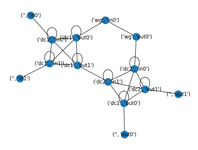
graph = sax.backends.additive._prune_internal_output_nodes(graph)
nx.draw_kamada_kawai(graph, with_labels=True)
We can now get a list of all possible paths in the network. Note that these paths must alternate between an S-edge and a C-edge:
paths = sax.backends.additive._get_possible_paths(graph, ("", "in0"), ("", "out0"))
paths
[[(('', 'in0'), ('dc1', 'in0')),
  (('dc1', 'in0'), ('dc1', 'out0')),
  (('dc1', 'out0'), ('wg', 'in0')),
  (('wg', 'in0'), ('wg', 'out0')),
  (('wg', 'out0'), ('dc2', 'in0')),
  (('dc2', 'in0'), ('dc2', 'out0')),
  (('dc2', 'out0'), ('', 'out0'))],
 [(('', 'in0'), ('dc1', 'in0')),
  (('dc1', 'in0'), ('dc1', 'out1')),
  (('dc1', 'out1'), ('dc2', 'in1')),
  (('dc2', 'in1'), ('dc2', 'out0')),
  (('dc2', 'out0'), ('', 'out0'))]]
And the path lengths of those paths can be calculated as follows:
sax.backends.additive._path_lengths(graph, paths)
[Array([101.41421356, 201.41421356, 301.41421356], dtype=float64),
 Array([0.], dtype=float64)]
This is all brought together in the additive KLU backend:
analyzed_instances = sax.backends.analyze_instances_additive(instances, models)
analyzed_circuit = sax.backends.analyze_circuit_additive(
    analyzed_instances, connections, ports
)
sax.backends.evaluate_circuit_additive(
    analyzed_circuit, {k: models[v["component"]]() for k, v in instances.items()}
)
/home/runner/work/sax/sax/.venv/lib/python3.12/site-packages/jax/_src/numpy/lax_numpy.py:5566: ComplexWarning: Casting complex values to real discards the imaginary part
  out_array: Array = lax_internal._convert_element_type(
{('in0', 'in0'): [Array([0.], dtype=float64)],
 ('in0',
  'in1'): [Array([101.41421356, 201.41421356, 301.41421356], dtype=float64), Array([100., 200., 300.], dtype=float64), Array([0.], dtype=float64)],
 ('in0',
  'out0'): [Array([101.41421356, 201.41421356, 301.41421356], dtype=float64), Array([0.], dtype=float64)],
 ('in0',
  'out1'): [Array([100.70710678, 200.70710678, 300.70710678], dtype=float64), Array([0.70710678], dtype=float64)],
 ('in1', 'in0'): [Array([100., 200., 300.], dtype=float64),
  Array([101.41421356, 201.41421356, 301.41421356], dtype=float64),
  Array([0.], dtype=float64)],
 ('in1', 'in1'): [Array([0.], dtype=float64)],
 ('in1',
  'out0'): [Array([100.70710678, 200.70710678, 300.70710678], dtype=float64), Array([0.70710678], dtype=float64)],
 ('in1', 'out1'): [Array([100., 200., 300.], dtype=float64),
  Array([1.41421356], dtype=float64)],
 ('out0',
  'in0'): [Array([101.41421356, 201.41421356, 301.41421356], dtype=float64), Array([0.], dtype=float64)],
 ('out0',
  'in1'): [Array([100.70710678, 200.70710678, 300.70710678], dtype=float64), Array([0.70710678], dtype=float64)],
 ('out0', 'out0'): [Array([0.], dtype=float64)],
 ('out0', 'out1'): [Array([0.], dtype=float64),
  Array([101.41421356, 201.41421356, 301.41421356], dtype=float64),
  Array([100., 200., 300.], dtype=float64)],
 ('out1',
  'in0'): [Array([100.70710678, 200.70710678, 300.70710678], dtype=float64), Array([0.70710678], dtype=float64)],
 ('out1', 'in1'): [Array([100., 200., 300.], dtype=float64),
  Array([1.41421356], dtype=float64)],
 ('out1', 'out0'): [Array([0.], dtype=float64),
  Array([100., 200., 300.], dtype=float64),
  Array([101.41421356, 201.41421356, 301.41421356], dtype=float64)],
 ('out1', 'out1'): [Array([0.], dtype=float64)]}