Thin film optimization#
Let’s optimize a thin film…
This notebook was contributed by simbilod.
import jax
import jax.example_libraries.optimizers as opt
import jax.numpy as jnp
import matplotlib.pyplot as plt
import sax
import tqdm.notebook as tqdm
from tmm import coh_tmm
In this notebook, we apply SAX to thin-film optimization and show how it can be used for wavelength-dependent parameter optimization.
The language of transfer/scatter matrices is commonly used to calculate optical properties of thin-films. Many specialized methods exist for their optimization. However, SAX can be useful to cut down on developer time by circumventing the need to manually take gradients of complicated or often-changed objective functions, and by generating efficient code from simple syntax.
Dielectric mirror Fabry-Pérot#
Consider a stack composed of only two materials, \(n_A\) and \(n_B\). Two types of transfer matrices characterize wave propagation in the system : interfaces described by Fresnel’s equations, and propagation.
For the two-material stack, this leads to 4 scatter matrices coefficients. Through reciprocity they can be constructed out of two independent ones :
def fresnel_mirror_ij(ni=1.0, nj=1.0):
    """Model a (fresnel) interface between twoo refractive indices

    Args:
        ni: refractive index of the initial medium
        nf: refractive index of the final
    """
    r_fresnel_ij = (ni - nj) / (ni + nj)  # i->j reflection
    t_fresnel_ij = 2 * ni / (ni + nj)  # i->j transmission
    r_fresnel_ji = -r_fresnel_ij  # j -> i reflection
    t_fresnel_ji = (1 - r_fresnel_ij**2) / t_fresnel_ij  # j -> i transmission
    sdict = {
        ("in", "in"): r_fresnel_ij,
        ("in", "out"): t_fresnel_ij,
        ("out", "in"): t_fresnel_ji,
        ("out", "out"): r_fresnel_ji,
    }
    return sdict


def propagation_i(ni=1.0, di=0.5, wl=0.532):
    """Model the phase shift acquired as a wave propagates through medium A

    Args:
        ni: refractive index of medium (at wavelength wl)
        di: [μm] thickness of layer
        wl: [μm] wavelength
    """
    prop_i = jnp.exp(1j * 2 * jnp.pi * ni * di / wl)
    sdict = {
        ("in", "out"): prop_i,
        ("out", "in"): prop_i,
    }
    return sdict
A resonant cavity can be formed when a high index region is surrounded by low-index region :
dielectric_fabry_perot, _ = sax.circuit(
    netlist={
        "instances": {
            "air_B": fresnel_mirror_ij,
            "B": propagation_i,
            "B_air": fresnel_mirror_ij,
        },
        "connections": {
            "air_B,out": "B,in",
            "B,out": "B_air,in",
        },
        "ports": {
            "in": "air_B,in",
            "out": "B_air,out",
        },
    },
    backend="fg",
)

settings = sax.get_settings(dielectric_fabry_perot)
settings
{'air_B': {'ni': 1.0, 'nj': 1.0},
 'B': {'ni': 1.0, 'di': 0.5, 'wl': 0.532},
 'B_air': {'ni': 1.0, 'nj': 1.0}}
Let’s choose \(n_A = 1\), \(n_B = 2\), \(d_B = 1000\) nm, and compute over the visible spectrum :
settings = sax.copy_settings(settings)
settings["air_B"]["nj"] = 2.0
settings["B"]["ni"] = 2.0
settings["B_air"]["ni"] = 2.0

wls = jnp.linspace(0.380, 0.750, 200)
settings = sax.update_settings(settings, wl=wls)
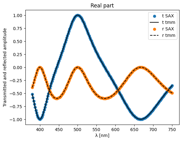
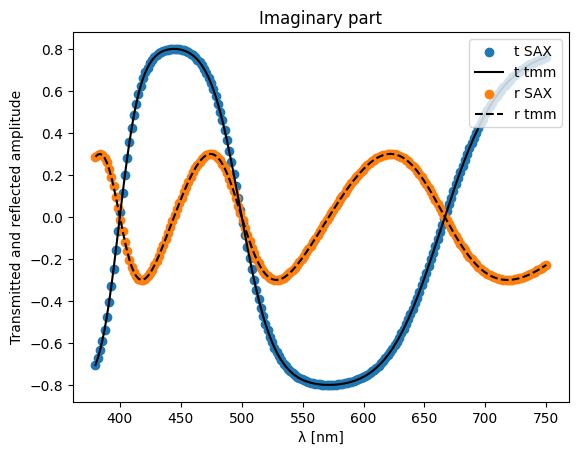
Compute transmission and reflection, and compare to another package’s results (https://github.com/sbyrnes321/tmm) :
%%time
sdict = dielectric_fabry_perot(**settings)

transmitted = sdict["in", "out"]
reflected = sdict["in", "in"]
CPU times: user 543 ms, sys: 17.9 ms, total: 561 ms
Wall time: 664 ms
%%time

# tmm syntax (https://github.com/sbyrnes321/tmm)
d_list = [jnp.inf, 0.500, jnp.inf]
n_list = [1, 2, 1]
# initialize lists of y-values to plot
rnorm = []
tnorm = []
Tnorm = []
Rnorm = []
for l in wls:
    rnorm.append(coh_tmm("s", n_list, d_list, 0, l)["r"])
    tnorm.append(coh_tmm("s", n_list, d_list, 0, l)["t"])
    Tnorm.append(coh_tmm("s", n_list, d_list, 0, l)["T"])
    Rnorm.append(coh_tmm("s", n_list, d_list, 0, l)["R"])
CPU times: user 1.07 s, sys: 15.3 ms, total: 1.08 s
Wall time: 1.09 s
plt.scatter(wls * 1e3, jnp.real(transmitted), label="t SAX")
plt.plot(wls * 1e3, jnp.real(jnp.array(tnorm)), "k", label="t tmm")
plt.scatter(wls * 1e3, jnp.real(reflected), label="r SAX")
plt.plot(wls * 1e3, jnp.real(jnp.array(rnorm)), "k--", label="r tmm")
plt.xlabel("λ [nm]")
plt.ylabel("Transmitted and reflected amplitude")
plt.legend(loc="upper right")
plt.title("Real part")
plt.show()

plt.scatter(wls * 1e3, jnp.imag(transmitted), label="t SAX")
plt.plot(wls * 1e3, jnp.imag(jnp.array(tnorm)), "k", label="t tmm")
plt.scatter(wls * 1e3, jnp.imag(reflected), label="r SAX")
plt.plot(wls * 1e3, jnp.imag(jnp.array(rnorm)), "k--", label="r tmm")
plt.xlabel("λ [nm]")
plt.ylabel("Transmitted and reflected amplitude")
plt.legend(loc="upper right")
plt.title("Imaginary part")
plt.show()
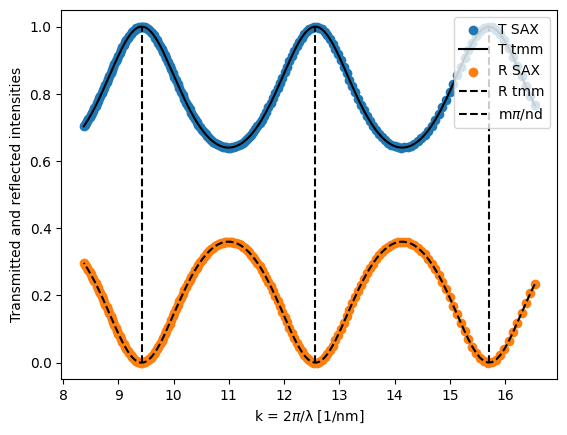
In terms of powers, we get the following. Due to the reflections at the interfaces, resonant behaviour is observed, with evenly-spaced maxima/minima in wavevector space :
plt.scatter(2 * jnp.pi / wls, jnp.abs(transmitted) ** 2, label="T SAX")
plt.plot(2 * jnp.pi / wls, Tnorm, "k", label="T tmm")
plt.scatter(2 * jnp.pi / wls, jnp.abs(reflected) ** 2, label="R SAX")
plt.plot(2 * jnp.pi / wls, Rnorm, "k--", label="R tmm")
plt.vlines(
    jnp.arange(3, 6) * jnp.pi / (2 * 0.5),
    ymin=0,
    ymax=1,
    color="k",
    linestyle="--",
    label=r"m$\pi$/nd",
)
plt.xlabel(r"k = 2$\pi$/λ [1/nm]")
plt.ylabel("Transmitted and reflected intensities")
plt.legend(loc="upper right")
plt.show()
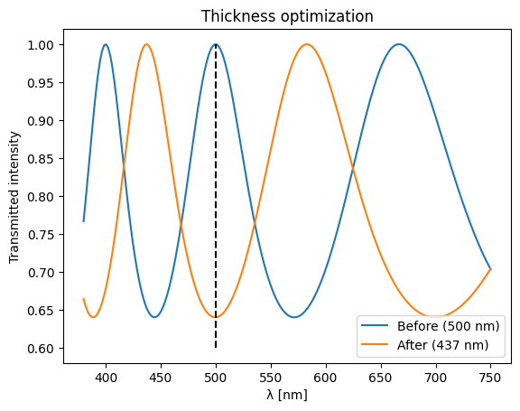
Optimization test#
Let’s attempt to minimize transmission at 500 nm by varying thickness.
@jax.jit
def loss(thickness):
    settings = sax.update_settings(sax.get_settings(dielectric_fabry_perot), wl=0.5)
    settings["B"]["di"] = thickness
    settings["air_B"]["nj"] = 2.0
    settings["B"]["ni"] = 2.0
    settings["B_air"]["ni"] = 2.0
    sdict = dielectric_fabry_perot(**settings)
    return jnp.abs(sdict["in", "out"]) ** 2
grad = jax.jit(jax.grad(loss))
initial_thickness = 0.5
optim_init, optim_update, optim_params = opt.adam(step_size=0.01)
optim_state = optim_init(initial_thickness)


def train_step(step, optim_state):
    thickness = optim_params(optim_state)
    lossvalue = loss(thickness)
    gradvalue = grad(thickness)
    optim_state = optim_update(step, gradvalue, optim_state)
    return lossvalue, optim_state
range_ = tqdm.trange(100)
for step in range_:
    lossvalue, optim_state = train_step(step, optim_state)
    range_.set_postfix(loss=f"{lossvalue:.6f}")
thickness = optim_params(optim_state)
thickness
Array(0.43726699, dtype=float64)
settings = sax.update_settings(sax.get_settings(dielectric_fabry_perot), wl=wls)
settings["B"]["di"] = thickness
settings["air_B"]["nj"] = 2.0
settings["B"]["ni"] = 2.0
settings["B_air"]["ni"] = 2.0
sdict = dielectric_fabry_perot(**settings)
detected = sdict["in", "out"]

plt.plot(wls * 1e3, jnp.abs(transmitted) ** 2, label="Before (500 nm)")
plt.plot(wls * 1e3, jnp.abs(detected) ** 2, label=f"After ({thickness*1e3:.0f} nm)")
plt.vlines(0.5 * 1e3, 0.6, 1, "k", linestyle="--")
plt.xlabel("λ [nm]")
plt.ylabel("Transmitted intensity")
plt.legend(loc="lower right")
plt.title("Thickness optimization")
plt.show()
General Fabry-Pérot étalon#
We reuse the propagation matrix above, and instead of simple interface matrices, model Fabry-Pérot mirrors as general lossless reciprocal scatter matrices :
For lossless reciprocal systems, we further have the requirements
and
The general Fabry-Pérot cavity is analytically described by :
def airy_t13(t12, t23, r21, r23, wl, d=1.0, n=1.0):
    """General Fabry-Pérot transmission transfer function (Airy formula)

    Args:
        t12 and r12 : S-parameters of the first mirror
        t23 and r23 : S-parameters of the second mirror
        wl : wavelength
        d : gap between the two mirrors (in units of wavelength)
        n : index of the gap between the two mirrors

    Returns:
        t13 : complex transmission amplitude of the mirror-gap-mirror system

    Note:
        Each mirror is assumed to be lossless and reciprocal : tij = tji, rij = rji
    """
    phi = n * 2 * jnp.pi * d / wl
    return t12 * t23 * jnp.exp(-1j * phi) / (1 - r21 * r23 * jnp.exp(-2j * phi))


def airy_r13(t12, t23, r21, r23, wl, d=1.0, n=1.0):
    """General Fabry-Pérot reflection transfer function (Airy formula)

    Args:
        t12 and r12 : S-parameters of the first mirror
        t23 and r23 : S-parameters of the second mirror
        wl : wavelength
        d : gap between the two mirrors (in units of wavelength)
        n : index of the gap between the two mirrors

    Returns:
        r13 : complex reflection amplitude of the mirror-gap-mirror system

    Note:
        Each mirror is assumed to be lossless and reciprocal : tij = tji, rij = rji
    """
    phi = n * 2 * jnp.pi * d / wl
    return r21 + t12 * t12 * r23 * jnp.exp(-2j * phi) / (
        1 - r21 * r23 * jnp.exp(-2j * phi)
    )
We need to implement the relationship between \(t\) and \(r\) for lossless reciprocal mirrors. The design parameter will be the amplitude and phase of the tranmission coefficient. The reflection coefficient is then fully determined :
def t_complex(t_amp, t_ang):
    return t_amp * jnp.exp(-1j * t_ang)


def r_complex(t_amp, t_ang):
    r_amp = jnp.sqrt((1.0 - t_amp**2))
    r_ang = t_ang - jnp.pi / 2
    return r_amp * jnp.exp(-1j * r_ang)
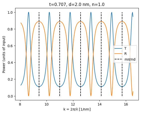
Let’s see the expected result for half-mirrors :
t_initial = jnp.sqrt(0.5)
d_gap = 2.0
n_gap = 1.0
r_initial = r_complex(t_initial, 0.0)

wls = jnp.linspace(0.38, 0.78, 500)

T_analytical_initial = (
    jnp.abs(airy_t13(t_initial, t_initial, r_initial, r_initial, wls, d=d_gap, n=n_gap))
    ** 2
)
R_analytical_initial = (
    jnp.abs(airy_r13(t_initial, t_initial, r_initial, r_initial, wls, d=d_gap, n=n_gap))
    ** 2
)

plt.title(f"t={t_initial:1.3f}, d={d_gap} nm, n={n_gap}")
plt.plot(2 * jnp.pi / wls, T_analytical_initial, label="T")
plt.plot(2 * jnp.pi / wls, R_analytical_initial, label="R")
plt.vlines(
    jnp.arange(6, 11) * jnp.pi / 2.0,
    ymin=0,
    ymax=1,
    color="k",
    linestyle="--",
    label=r"m$\pi$/nd",
)
plt.xlabel(r"k = 2$\pi$/$\lambda$ [1/nm]")
plt.ylabel("Power (units of input)")
plt.legend()
plt.show()

plt.title(f"t={t_initial:1.3f}, d={d_gap} nm, n={n_gap}")
plt.plot(wls * 1e3, T_analytical_initial, label="T")
plt.plot(wls * 1e3, R_analytical_initial, label="R")
plt.xlabel(r"$\lambda$ (nm)")
plt.ylabel("Power (units of input)")
plt.legend()
plt.show()
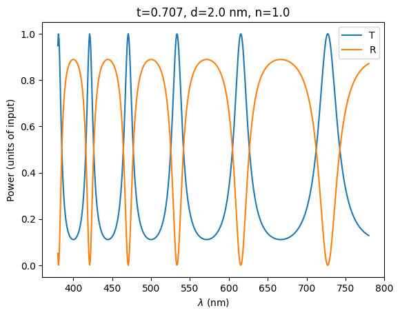
# Is power conserved? (to within 0.1%)
assert jnp.isclose(R_analytical_initial + T_analytical_initial, 1, 0.001).all()
Now let’s do the same with SAX by defining new elements :
def mirror(t_amp=0.5**0.5, t_ang=0.0):
    r_complex_val = r_complex(t_amp, t_ang)
    t_complex_val = t_complex(t_amp, t_ang)
    sdict = {
        ("in", "in"): r_complex_val,
        ("in", "out"): t_complex_val,
        ("out", "in"): t_complex_val,  # (1 - r_complex_val**2)/t_complex_val, # t_ji
        ("out", "out"): r_complex_val,  # -r_complex_val, # r_ji
    }
    return sdict


fabry_perot_tunable, _ = sax.circuit(
    netlist={
        "instances": {
            "mirror1": mirror,
            "gap": propagation_i,
            "mirror2": mirror,
        },
        "connections": {
            "mirror1,out": "gap,in",
            "gap,out": "mirror2,in",
        },
        "ports": {
            "in": "mirror1,in",
            "out": "mirror2,out",
        },
    },
    backend="fg",
)

settings = sax.get_settings(fabry_perot_tunable)
settings
{'mirror1': {'t_amp': 0.7071067811865476, 't_ang': 0.0},
 'gap': {'ni': 1.0, 'di': 0.5, 'wl': 0.532},
 'mirror2': {'t_amp': 0.7071067811865476, 't_ang': 0.0}}
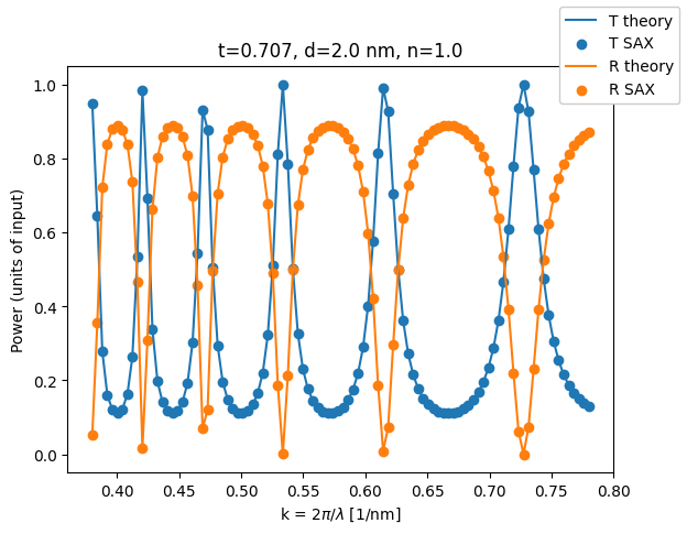
N = 100
wls = jnp.linspace(0.38, 0.78, N)
settings = sax.get_settings(fabry_perot_tunable)
settings = sax.update_settings(settings, wl=wls, t_amp=jnp.sqrt(0.5), t_ang=0.0)
settings["gap"]["ni"] = 1.0
settings["gap"]["di"] = 2.0
transmitted_initial = fabry_perot_tunable(**settings)["in", "out"]
reflected_initial = fabry_perot_tunable(**settings)["out", "out"]
T_analytical_initial = (
    jnp.abs(airy_t13(t_initial, t_initial, r_initial, r_initial, wls, d=d_gap, n=n_gap))
    ** 2
)
R_analytical_initial = (
    jnp.abs(airy_r13(t_initial, t_initial, r_initial, r_initial, wls, d=d_gap, n=n_gap))
    ** 2
)
plt.title(f"t={t_initial:1.3f}, d={d_gap} nm, n={n_gap}")
plt.plot(wls, T_analytical_initial, label="T theory")
plt.scatter(wls, jnp.abs(transmitted_initial) ** 2, label="T SAX")
plt.plot(wls, R_analytical_initial, label="R theory")
plt.scatter(wls, jnp.abs(reflected_initial) ** 2, label="R SAX")
plt.xlabel(r"k = 2$\pi$/$\lambda$ [1/nm]")
plt.ylabel("Power (units of input)")
plt.figlegend(framealpha=1.0)
plt.show()
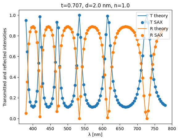
Wavelength-dependent Fabry-Pérot étalon#
Let’s repeat with a model where parameters can be wavelength-dependent. To comply with the optimizer object, we will stack all design parameters in a single array :
ts_initial = jnp.zeros(2 * N)
ts_initial = ts_initial.at[0:N].set(jnp.sqrt(0.5))
We will simply loop over all wavelengths, and use different \(t\) parameters at each wavelength.
wls = jnp.linspace(0.38, 0.78, N)
transmitted = jnp.zeros_like(wls)
reflected = jnp.zeros_like(wls)
settings = sax.get_settings(fabry_perot_tunable)
settings = sax.update_settings(
    settings, wl=wls, t_amp=ts_initial[:N], t_ang=ts_initial[N:]
)
settings["gap"]["ni"] = 1.0
settings["gap"]["di"] = 2.0
# Perform computation
sdict = fabry_perot_tunable(**settings)
transmitted = jnp.abs(sdict["in", "out"]) ** 2
reflected = jnp.abs(sdict["in", "in"]) ** 2
plt.plot(wls * 1e3, T_analytical_initial, label="T theory")
plt.scatter(wls * 1e3, transmitted, label="T SAX")
plt.plot(wls * 1e3, R_analytical_initial, label="R theory")
plt.scatter(wls * 1e3, reflected, label="R SAX")
plt.xlabel("λ [nm]")
plt.ylabel("Transmitted and reflected intensities")
plt.legend(loc="upper right")
plt.title(f"t={t_initial:1.3f}, d={d_gap} nm, n={n_gap}")
plt.show()
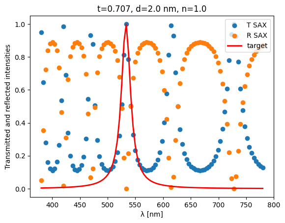
Since it seems to work, let’s add a target and optimize some harmonics away :
def lorentzian(l0, dl, wl, A):
    return A / ((wl - l0) ** 2 + (0.5 * dl) ** 2)


target = lorentzian(533.0, 20.0, wls * 1e3, 100.0)

plt.scatter(wls * 1e3, transmitted, label="T SAX")
plt.scatter(wls * 1e3, reflected, label="R SAX")
plt.plot(wls * 1e3, target, "r", linewidth=2, label="target")
plt.xlabel("λ [nm]")
plt.ylabel("Transmitted and reflected intensities")
plt.legend(loc="upper right")
plt.title(f"t={t_initial:1.3f}, d={d_gap} nm, n={n_gap}")
plt.show()
@jax.jit
def loss(ts):
    N = len(ts[::2])
    wls = jnp.linspace(0.38, 0.78, N)
    target = lorentzian(533.0, 20.0, wls * 1e3, 100.0)
    settings = sax.get_settings(fabry_perot_tunable)
    settings = sax.update_settings(settings, wl=wls, t_amp=ts[:N], t_ang=ts[N:])
    settings["gap"]["ni"] = 1.0
    settings["gap"]["di"] = 2.0
    sdict = fabry_perot_tunable(**settings)
    transmitted = jnp.abs(sdict["in", "out"]) ** 2
    return (jnp.abs(transmitted - target) ** 2).mean()
grad = jax.jit(jax.grad(loss))
optim_init, optim_update, optim_params = opt.adam(step_size=0.01)


def train_step(step, optim_state):
    ts = optim_params(optim_state)
    lossvalue = loss(ts)
    gradvalue = grad(ts)
    optim_state = optim_update(step, gradvalue, optim_state)
    return lossvalue, gradvalue, optim_state
range_ = tqdm.trange(200)

optim_state = optim_init(ts_initial)
for step in range_:
    lossvalue, gradvalue, optim_state = train_step(step, optim_state)
    range_.set_postfix(loss=f"{lossvalue:.6f}")
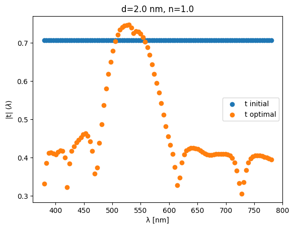
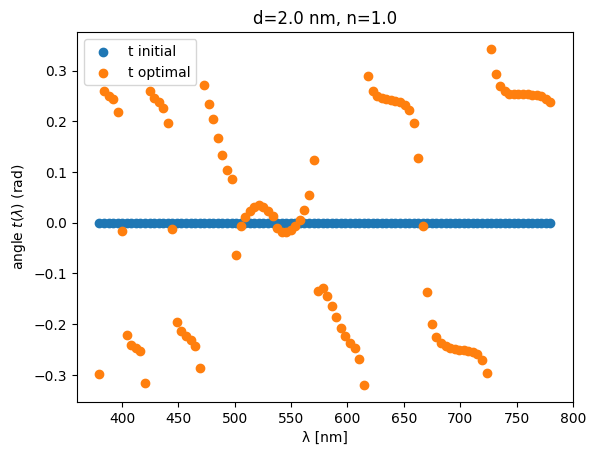
The optimized parameters are now wavelength-dependent :
ts_optimal = optim_params(optim_state)

plt.scatter(wls * 1e3, ts_initial[:N], label="t initial")
plt.scatter(wls * 1e3, ts_optimal[:N], label="t optimal")
plt.xlabel("λ [nm]")
plt.ylabel(r"|t| $(\lambda)$")
plt.legend(loc="best")
plt.title(f"d={d_gap} nm, n={n_gap}")
plt.show()

plt.scatter(wls * 1e3, ts_initial[N:], label="t initial")
plt.scatter(wls * 1e3, ts_optimal[N:], label="t optimal")
plt.xlabel("λ [nm]")
plt.ylabel(r"angle $t (\lambda)$ (rad)")
plt.legend(loc="best")
plt.title(f"d={d_gap} nm, n={n_gap}")
plt.show()
Visualizing the result :
wls = jnp.linspace(0.38, 0.78, N)
transmitted_optimal = jnp.zeros_like(wls)
reflected_optimal = jnp.zeros_like(wls)

settings = sax.get_settings(fabry_perot_tunable)
settings = sax.update_settings(
    settings, wl=wls, t_amp=ts_optimal[:N], t_ang=ts_optimal[N:]
)
settings["gap"]["ni"] = 1.0
settings["gap"]["di"] = 2.0
transmitted_optimal = jnp.abs(fabry_perot_tunable(**settings)["in", "out"]) ** 2
reflected_optimal = jnp.abs(fabry_perot_tunable(**settings)["in", "in"]) ** 2
plt.scatter(wls * 1e3, transmitted_optimal, label="T")
plt.scatter(wls * 1e3, reflected_optimal, label="R")
plt.plot(wls * 1e3, lorentzian(533, 20, wls * 1e3, 100), "r", label="target")
plt.xlabel("λ [nm]")
plt.ylabel("Transmitted and reflected intensities")
plt.legend(loc="upper right")
plt.title(r"Optimized t($\lambda$), " + f"d={d_gap} nm, n={n_gap}")
plt.show()
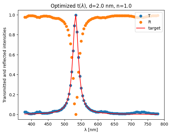
The hard part is now to find physical stacks that physically implement \(t(\lambda)\). However, the ease with which we can modify and complexify the loss function opens opportunities for regularization and more complicated objective functions.
The models above are available in sax.models.thinfilm, and can straightforwardly be extended to propagation at an angle, s and p polarizations, nonreciprocal systems, and systems with losses.