Circuit#
SAX Circuits
from functools import partial

import sax
from sax.circuit import (
    _create_dag,
    _find_leaves,
    _find_root,
    _flat_circuit,
    _validate_models,
    draw_dag,
)
Let’s start by creating a simple recursive netlist with gdsfactory.
Note
We are using gdsfactory to create our netlist because it allows us to see the circuit we want to simulate and because we’re striving to have a compatible netlist implementation in SAX.
However… gdsfactory is not a dependency of SAX. You can also define your circuits by hand (see SAX Quick Start or you can use another tool to programmatically construct your netlists.
import gdsfactory as gf
from IPython.display import display
from gdsfactory.components import mzi
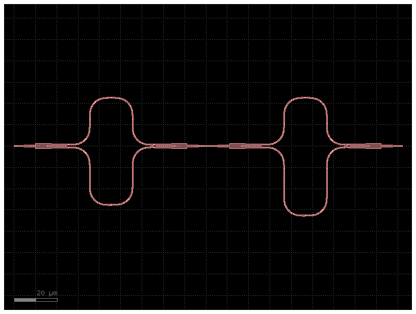
@gf.cell
def twomzi():
c = gf.Component()
# instances
mzi1 = mzi(delta_length=10)
mzi2 = mzi(delta_length=20)
# references
mzi1_ = c.add_ref(mzi1, name="mzi1")
mzi2_ = c.add_ref(mzi2, name="mzi2")
# connections
mzi2_.connect("o1", mzi1_.ports["o2"])
# ports
c.add_port("o1", port=mzi1_.ports["o1"])
c.add_port("o2", port=mzi2_.ports["o2"])
return c
comp = twomzi()
comp
recnet = sax.RecursiveNetlist.parse_obj(comp.get_netlist(recursive=True))
mzi1_comp = recnet.root["twomzi"].instances["mzi1"].component
flatnet = recnet.root[mzi1_comp]
/tmp/ipykernel_4232/418843444.py:1: PydanticDeprecatedSince20: The `parse_obj` method is deprecated; use `model_validate` instead. Deprecated in Pydantic V2.0 to be removed in V3.0. See Pydantic V2 Migration Guide at https://errors.pydantic.dev/2.10/migration/
  recnet = sax.RecursiveNetlist.parse_obj(comp.get_netlist(recursive=True))
To be able to model this device we’ll need some SAX dummy models:
def bend_euler(
    angle=90.0,
    p=0.5,
    # cross_section="strip",
    # direction="ccw",
    # with_bbox=True,
    # with_arc_floorplan=True,
    # npoints=720,
):
    return sax.reciprocal({("o1", "o2"): 1.0})
def mmi1x2(
    width=0.5,
    width_taper=1.0,
    length_taper=10.0,
    length_mmi=5.5,
    width_mmi=2.5,
    gap_mmi=0.25,
    # cross_section= strip,
    # taper= {function= taper},
    # with_bbox= True,
):
    return sax.reciprocal(
        {
            ("o1", "o2"): 0.45**0.5,
            ("o1", "o3"): 0.45**0.5,
        }
    )
def mmi2x2(
    width=0.5,
    width_taper=1.0,
    length_taper=10.0,
    length_mmi=5.5,
    width_mmi=2.5,
    gap_mmi=0.25,
    # cross_section= strip,
    # taper= {function= taper},
    # with_bbox= True,
):
    return sax.reciprocal(
        {
            ("o1", "o3"): 0.45**0.5,
            ("o1", "o4"): 1j * 0.45**0.5,
            ("o2", "o3"): 1j * 0.45**0.5,
            ("o2", "o4"): 0.45**0.5,
        }
    )
def straight(
    length=0.01,
    # npoints=2,
    # with_bbox=True,
    # cross_section=...
):
    return sax.reciprocal({("o1", "o2"): 1.0})
In SAX, we usually aggregate the available models in a models dictionary:
models = {
    "straight": straight,
    "bend_euler": bend_euler,
    "mmi1x2": mmi1x2,
}
We can also create some dummy multimode models:
def bend_euler_mm(
    angle=90.0,
    p=0.5,
    # cross_section="strip",
    # direction="ccw",
    # with_bbox=True,
    # with_arc_floorplan=True,
    # npoints=720,
):
    return sax.reciprocal(
        {
            ("o1@TE", "o2@TE"): 0.9**0.5,
            # ('o1@TE', 'o2@TM'): 0.01**0.5,
            # ('o1@TM', 'o2@TE'): 0.01**0.5,
            ("o1@TM", "o2@TM"): 0.8**0.5,
        }
    )
def mmi1x2_mm(
    width=0.5,
    width_taper=1.0,
    length_taper=10.0,
    length_mmi=5.5,
    width_mmi=2.5,
    gap_mmi=0.25,
    # cross_section= strip,
    # taper= {function= taper},
    # with_bbox= True,
):
    return sax.reciprocal(
        {
            ("o1@TE", "o2@TE"): 0.45**0.5,
            ("o1@TE", "o3@TE"): 0.45**0.5,
            ("o1@TM", "o2@TM"): 0.41**0.5,
            ("o1@TM", "o3@TM"): 0.41**0.5,
            ("o1@TE", "o2@TM"): 0.01**0.5,
            ("o1@TM", "o2@TE"): 0.01**0.5,
            ("o1@TE", "o3@TM"): 0.02**0.5,
            ("o1@TM", "o3@TE"): 0.02**0.5,
        }
    )
def straight_mm(
    length=0.01,
    # npoints=2,
    # with_bbox=True,
    # cross_section=...
):
    return sax.reciprocal(
        {
            ("o1@TE", "o2@TE"): 1.0,
            ("o1@TM", "o2@TM"): 1.0,
        }
    )
models_mm = {
    "straight": straight_mm,
    "bend_euler": bend_euler_mm,
    "mmi1x2": mmi1x2_mm,
}
We can now represent our recursive netlist model as a Directed Acyclic Graph:
dag = _create_dag(recnet, models)
draw_dag(dag)
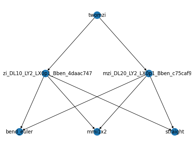
Note that the DAG depends on the models we supply. We could for example stub one of the sub-netlists by a pre-defined model:
dag_ = _create_dag(recnet, {**models, "mzi_delta_length10": mmi2x2})
draw_dag(dag_, with_labels=True)
This is useful if we for example pre-calculated a certain model.
We can easily find the root of the DAG:
_find_root(dag)
['twomzi']
Similarly we can find the leaves:
_find_leaves(dag)
['bend_euler', 'mmi1x2', 'straight']
To be able to simulate the circuit, we need to supply a model for each of the leaves in the dependency DAG. Let’s write a validator that checks this
models = _validate_models(models, dag)
We can now dow a bottom-up simulation. Since at the bottom of the DAG, our circuit is always flat (i.e. not hierarchical) we can implement a minimal _flat_circuit definition, which only needs to work on a flat (non-hierarchical circuit):
flatnet = recnet.root[mzi1_comp]
single_mzi = _flat_circuit(
    flatnet.instances,
    flatnet.connections,
    flatnet.ports,
    models,
    "default",
)
single_mzi()
(Array([[0. +0.j, 0.9+0.j],
        [0.9+0.j, 0. +0.j]], dtype=complex128),
 {'o1': 0, 'o2': 1})
The resulting circuit is just another SAX model (i.e. a python function) returing an SType:
?single_mzi
Let’s ‘execute’ the circuit:
Note that we can also supply multimode models:
flatnet = recnet.root[mzi1_comp]
single_mzi = _flat_circuit(
    flatnet.instances,
    flatnet.connections,
    flatnet.ports,
    models_mm,
    "default",
)
single_mzi()
(Array([[0.        +0.j, 0.        +0.j, 0.7482    +0.j, 0.23011426+0.j],
        [0.        +0.j, 0.        +0.j, 0.23011426+0.j, 0.5491    +0.j],
        [0.7482    +0.j, 0.23011426+0.j, 0.        +0.j, 0.        +0.j],
        [0.23011426+0.j, 0.5491    +0.j, 0.        +0.j, 0.        +0.j]],      dtype=complex128),
 {'o1@TE': 0, 'o1@TM': 1, 'o2@TE': 2, 'o2@TM': 3})
Now that we can handle flat circuits the extension to hierarchical circuits is not so difficult:
single mode simulation:
double_mzi, info = sax.circuit(recnet, models, backend="default")
double_mzi()
/home/runner/work/sax/sax/.venv/lib/python3.12/site-packages/jax/_src/numpy/lax_numpy.py:5732: FutureWarning: None encountered in jnp.array(); this is currently treated as NaN. In the future this will result in an error.
  return array(a, dtype=dtype, copy=bool(copy), order=order, device=device)
/home/runner/work/sax/sax/.venv/lib/python3.12/site-packages/jax/_src/numpy/lax_numpy.py:5732: FutureWarning: None encountered in jnp.array(); this is currently treated as NaN. In the future this will result in an error.
  return array(a, dtype=dtype, copy=bool(copy), order=order, device=device)
/home/runner/work/sax/sax/.venv/lib/python3.12/site-packages/jax/_src/numpy/lax_numpy.py:5732: FutureWarning: None encountered in jnp.array(); this is currently treated as NaN. In the future this will result in an error.
  return array(a, dtype=dtype, copy=bool(copy), order=order, device=device)
/home/runner/work/sax/sax/.venv/lib/python3.12/site-packages/jax/_src/numpy/lax_numpy.py:5732: FutureWarning: None encountered in jnp.array(); this is currently treated as NaN. In the future this will result in an error.
  return array(a, dtype=dtype, copy=bool(copy), order=order, device=device)
{('o1', 'o1'): Array(0.+0.j, dtype=complex128),
 ('o1', 'o2'): Array(0.81+0.j, dtype=complex128),
 ('o2', 'o1'): Array(0.81+0.j, dtype=complex128),
 ('o2', 'o2'): Array(0.+0.j, dtype=complex128)}
multi mode simulation:
double_mzi, info = sax.circuit(
    recnet, models_mm, backend="default", return_type="sdict"
)
double_mzi()
/home/runner/work/sax/sax/.venv/lib/python3.12/site-packages/jax/_src/numpy/lax_numpy.py:5732: FutureWarning: None encountered in jnp.array(); this is currently treated as NaN. In the future this will result in an error.
  return array(a, dtype=dtype, copy=bool(copy), order=order, device=device)
/home/runner/work/sax/sax/.venv/lib/python3.12/site-packages/jax/_src/numpy/lax_numpy.py:5732: FutureWarning: None encountered in jnp.array(); this is currently treated as NaN. In the future this will result in an error.
  return array(a, dtype=dtype, copy=bool(copy), order=order, device=device)
/home/runner/work/sax/sax/.venv/lib/python3.12/site-packages/jax/_src/numpy/lax_numpy.py:5732: FutureWarning: None encountered in jnp.array(); this is currently treated as NaN. In the future this will result in an error.
  return array(a, dtype=dtype, copy=bool(copy), order=order, device=device)
/home/runner/work/sax/sax/.venv/lib/python3.12/site-packages/jax/_src/numpy/lax_numpy.py:5732: FutureWarning: None encountered in jnp.array(); this is currently treated as NaN. In the future this will result in an error.
  return array(a, dtype=dtype, copy=bool(copy), order=order, device=device)
{('o1@TE', 'o1@TE'): Array(0.+0.j, dtype=complex128),
 ('o1@TE', 'o1@TM'): Array(0.+0.j, dtype=complex128),
 ('o1@TE', 'o2@TE'): Array(0.61275581+0.j, dtype=complex128),
 ('o1@TE', 'o2@TM'): Array(0.29852723+0.j, dtype=complex128),
 ('o1@TM', 'o1@TE'): Array(0.+0.j, dtype=complex128),
 ('o1@TM', 'o1@TM'): Array(0.+0.j, dtype=complex128),
 ('o1@TM', 'o2@TE'): Array(0.29852723+0.j, dtype=complex128),
 ('o1@TM', 'o2@TM'): Array(0.35446338+0.j, dtype=complex128),
 ('o2@TE', 'o1@TE'): Array(0.61275581+0.j, dtype=complex128),
 ('o2@TE', 'o1@TM'): Array(0.29852723+0.j, dtype=complex128),
 ('o2@TE', 'o2@TE'): Array(0.+0.j, dtype=complex128),
 ('o2@TE', 'o2@TM'): Array(0.+0.j, dtype=complex128),
 ('o2@TM', 'o1@TE'): Array(0.29852723+0.j, dtype=complex128),
 ('o2@TM', 'o1@TM'): Array(0.35446338+0.j, dtype=complex128),
 ('o2@TM', 'o2@TE'): Array(0.+0.j, dtype=complex128),
 ('o2@TM', 'o2@TM'): Array(0.+0.j, dtype=complex128)}
sometimes it’s useful to get the required circuit model names to be able to create the circuit:
sax.get_required_circuit_models(recnet, models)
['bend_euler', 'mmi1x2', 'straight']