Probes

Measure intermediate signals in circuits using ideal measurement probes.

Introduction

When debugging or analyzing complex circuits, it's often useful to observe the signal at intermediate points—not just at the external ports. SAX provides a [probes][sax.models.probes] feature that allows you to insert ideal measurement taps at any connection point in your circuit.

Each probe is an unphysical 4-port device with: - 100% transmission through the main path - 100% coupling to forward and backward tap ports

This allows you to "see" what's happening inside your circuit without affecting the signal propagation.

Imports

import jax.numpy as jnp
import matplotlib.pyplot as plt

import sax

Define Component Models

Let's define simple coupler and waveguide models, similar to the quick start example:

def coupler(coupling=0.5) -> sax.SDict:
    kappa = coupling**0.5
    tau = (1 - coupling) ** 0.5
    return sax.reciprocal(
        {
            ("in0", "out0"): tau,
            ("in0", "out1"): 1j * kappa,
            ("in1", "out0"): 1j * kappa,
            ("in1", "out1"): tau,
        }
    )


def waveguide(wl=1.55, wl0=1.55, neff=2.34, ng=3.4, length=10.0, loss=0.0) -> sax.SDict:
    dwl = wl - wl0
    dneff_dwl = (ng - neff) / wl0
    neff = neff - dwl * dneff_dwl
    phase = 2 * jnp.pi * neff * length / wl
    transmission = 10 ** (-loss * length / 20) * jnp.exp(1j * phase)
    return sax.reciprocal(
        {
            ("in0", "out0"): transmission,
        }
    )

MZI Circuit

Now let's create a Mach-Zehnder Interferometer (MZI) circuit:

        _________
       |   top   |
in0 ---+---------+--- out0
       |         |
in1 ---+---------+--- out1
       |___btm___|

mzi_netlist = {
    "instances": {
        "lft": "coupler",
        "top": "waveguide",
        "btm": "waveguide",
        "rgt": "coupler",
    },
    "connections": {
        "lft,out0": "btm,in0",
        "btm,out0": "rgt,in0",
        "lft,out1": "top,in0",
        "top,out0": "rgt,in1",
    },
    "ports": {
        "in0": "lft,in0",
        "in1": "lft,in1",
        "out0": "rgt,out0",
        "out1": "rgt,out1",
    },
}

models = {
    "coupler": coupler,
    "waveguide": waveguide,
}

Adding Probes

To observe the signal at intermediate points, we can add probes using the [probes][sax.models.probes] argument to sax.circuit(). Each probe is specified as a mapping from probe name to instance port.

Let's add probes to measure the signal in both arms of the MZI:

mzi_with_probes, info = sax.circuit(
    netlist=mzi_netlist,
    models=models,
    probes={
        "top_arm": "top,in0",  # Probe at the input of the top waveguide
        "btm_arm": "btm,in0",  # Probe at the input of the bottom waveguide
    },
)

The circuit now has additional ports for each probe. Each probe creates two ports: - {name}_fwd: Signal flowing into the probed port - {name}_bwd: Signal flowing out of the probed port

S = mzi_with_probes()
ports = sax.get_ports(S)
print("Circuit ports:", ports)

Circuit ports: ('btm_arm_bwd', 'btm_arm_fwd', 'in0', 'in1', 'out0', 'out1', 'top_arm_bwd', 'top_arm_fwd')

Simulating with Probes

Let's simulate the MZI with different arm lengths and observe the signal at the probe points:

wl = jnp.linspace(1.5, 1.6, 1000)

S = mzi_with_probes(
    wl=wl,
    top={"length": 25.0},
    btm={"length": 15.0},
)

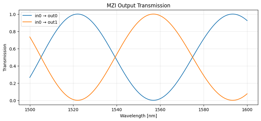
Output Transmission

First, let's look at the standard output transmission:

plt.figure(figsize=(10, 4))
plt.plot(wl * 1e3, jnp.abs(S["in0", "out0"]) ** 2, label="in0 → out0")
plt.plot(wl * 1e3, jnp.abs(S["in0", "out1"]) ** 2, label="in0 → out1")
plt.xlabel("Wavelength [nm]")
plt.ylabel("Transmission")
plt.title("MZI Output Transmission")
plt.legend()
plt.ylim(-0.05, 1.05)
plt.grid(True, alpha=0.3)
plt.show()

Signal at Probe Points

Now let's look at the signal entering each arm of the MZI. The _fwd ports show us the signal flowing into the probed ports:

plt.figure(figsize=(10, 4))
plt.plot(wl * 1e3, jnp.abs(S["in0", "top_arm_fwd"]) ** 2, label="in0 → top arm (fwd)")
plt.plot(wl * 1e3, jnp.abs(S["in0", "btm_arm_fwd"]) ** 2, label="in0 → btm arm (fwd)", ls="--")  # fmt: skip
plt.xlabel("Wavelength [nm]")
plt.ylabel("Power")
plt.title("Signal Entering Each Arm (from in0)")
plt.legend()
plt.ylim(-0.05, 1.05)
plt.grid(True, alpha=0.3)
plt.show()

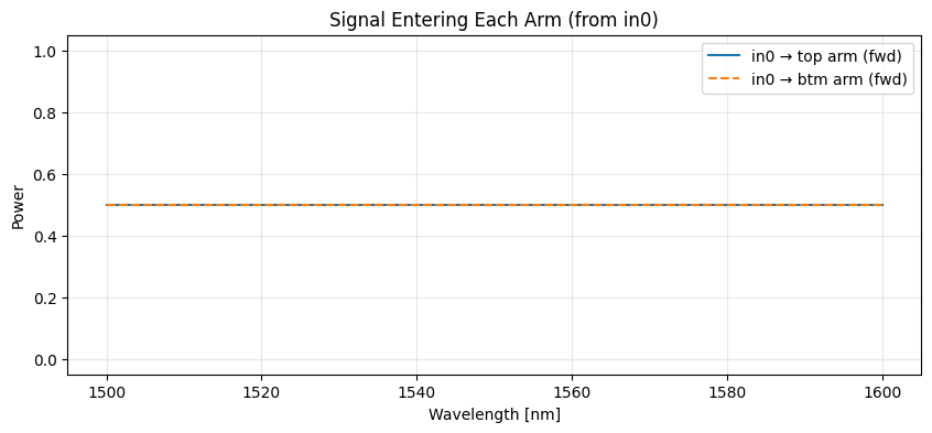
As expected with a 50/50 coupler, the signal is split equally between the two arms.

Probes Don't Affect Circuit Behavior

An important property of probes is that they don't affect the circuit's behavior. Let's verify this by comparing with a circuit without probes:

# Circuit without probes
mzi_no_probes, _ = sax.circuit(netlist=mzi_netlist, models=models)

S_no_probes = mzi_no_probes(wl=wl, top={"length": 25.0}, btm={"length": 15.0})

# Compare outputs
diff = jnp.abs(S["in0", "out0"] - S_no_probes["in0", "out0"])
print(f"Maximum difference in transmission: {jnp.max(diff):.2e}")

Maximum difference in transmission: 0.00e+00

The outputs are identical (within numerical precision), confirming that probes are purely observational.

Summary

The [probes][sax.models.probes] feature in SAX allows you to:

1. Observe intermediate signals without modifying your netlist
2. Debug circuit behavior by seeing what happens inside
3. Analyze both forward and backward propagating waves at any connection point
4. Access phase information for understanding interference

Key points: - Probes are specified as probes={"name": "instance,port"} in sax.circuit() - Each probe creates {name}_fwd and {name}_bwd ports - _fwd captures signal flowing into the specified port - _bwd captures signal flowing out of the specified port - Probes are unphysical (they don't conserve energy) but don't affect circuit behavior

Ports as probes

When a port is applied on an internal node (i.e., an instance port that is already part of a connection) it usually is ignored, however we can also make it it automatically be interpreted as a probe:

mzi_netlist = {
    "instances": {
        "lft": "coupler",
        "top": "waveguide",
        "btm": "waveguide",
        "rgt": "coupler",
    },
    "connections": {
        "lft,out0": "btm,in0",
        "btm,out0": "rgt,in0",
        "lft,out1": "top,in0",
        "top,out0": "rgt,in1",
    },
    "ports": {
        "in0": "lft,in0",
        "in1": "lft,in1",
        "out0": "rgt,out0",
        "out1": "rgt,out1",
        "top_arm": "top,in0",  # Internal node -> interpreted as probe
        "btm_arm": "btm,in0",  # Internal node -> interpreted as probe
    },
}

models = {
    "coupler": coupler,
    "waveguide": waveguide,
}

circuit, _ = sax.circuit(mzi_netlist, models, on_internal_port="as_probes")

S = circuit(
    wl=wl,
    top={"length": 25.0},
    btm={"length": 15.0},
)
ports = sax.get_ports(S)
print(f"Circuit ports: {ports}")

Circuit ports: ('btm_arm_bwd', 'btm_arm_fwd', 'in0', 'in1', 'out0', 'out1', 'top_arm_bwd', 'top_arm_fwd')


/home/runner/work/sax/sax/src/sax/netlists.py:711: UserWarning: Port 'top_arm' maps to internal node 'top,in0' which is already part of a connection. It will be interpreted as a probe (creating 'top_arm_fwd' and 'top_arm_bwd' ports).
  modified_top, probes = extract_port_probes(top_level, on_internal_port)
/home/runner/work/sax/sax/src/sax/netlists.py:711: UserWarning: Port 'btm_arm' maps to internal node 'btm,in0' which is already part of a connection. It will be interpreted as a probe (creating 'btm_arm_fwd' and 'btm_arm_bwd' ports).
  modified_top, probes = extract_port_probes(top_level, on_internal_port)

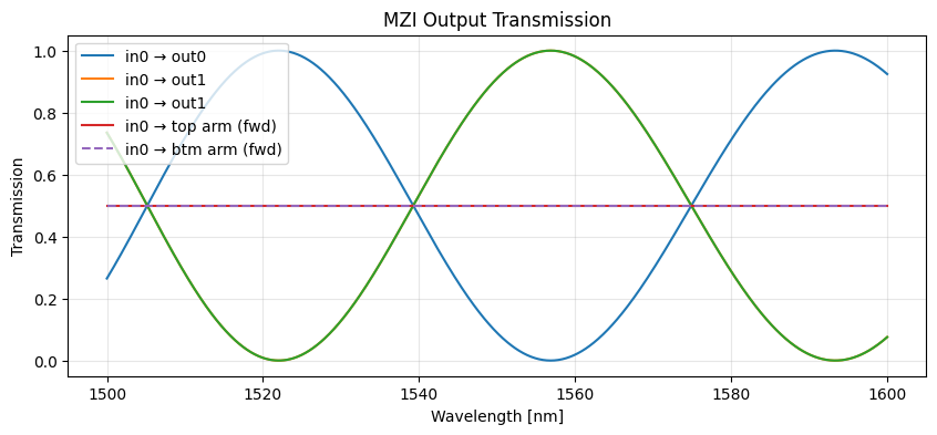
plt.figure(figsize=(10, 4))
plt.plot(wl * 1e3, jnp.abs(S["in0", "out0"]) ** 2, label="in0 → out0")
plt.plot(wl * 1e3, jnp.abs(S["in0", "out1"]) ** 2, label="in0 → out1")
plt.plot(wl * 1e3, jnp.abs(S["in0", "out1"]) ** 2, label="in0 → out1")
plt.plot(wl * 1e3, jnp.abs(S["in0", "top_arm_fwd"]) ** 2, label="in0 → top arm (fwd)")
plt.plot(wl * 1e3, jnp.abs(S["in0", "btm_arm_fwd"]) ** 2, label="in0 → btm arm (fwd)", ls="--")  # fmt: skip
plt.xlabel("Wavelength [nm]")
plt.ylabel("Transmission")
plt.title("MZI Output Transmission")
plt.legend()
plt.ylim(-0.05, 1.05)
plt.grid(True, alpha=0.3)
plt.show()

Hierarchical Probes

Probes can also target instance ports inside sub-circuits using dot-separated paths. For example, "mzi.top,in0" probes port in0 of instance top inside the component used by instance mzi.

The probe ports (_fwd and _bwd) are automatically exposed through every level of the hierarchy.

hierarchical_netlist = {
    "top_level": {
        "instances": {
            "mzi": "mzi_component",
        },
        "connections": {},
        "ports": {
            "in0": "mzi,in0",
            "in1": "mzi,in1",
            "out0": "mzi,out0",
            "out1": "mzi,out1",
        },
    },
    "mzi_component": {
        "instances": {
            "lft": "coupler",
            "top": "waveguide",
            "btm": "waveguide",
            "rgt": "coupler",
        },
        "connections": {
            "lft,out0": "btm,in0",
            "btm,out0": "rgt,in0",
            "lft,out1": "top,in0",
            "top,out0": "rgt,in1",
        },
        "ports": {
            "in0": "lft,in0",
            "in1": "lft,in1",
            "out0": "rgt,out0",
            "out1": "rgt,out1",
        },
    },
}

mzi_hier, _ = sax.circuit(
    hierarchical_netlist,
    models,
    probes={
        "top_arm": "mzi.top,in0",
        "btm_arm": "mzi.btm,in0",
    },
)

S = mzi_hier(wl=wl, mzi={"top": {"length": 25.0}, "btm": {"length": 15.0}})
print("Circuit ports:", sax.get_ports(S))

Circuit ports: ('btm_arm_bwd', 'btm_arm_fwd', 'in0', 'in1', 'out0', 'out1', 'top_arm_bwd', 'top_arm_fwd')

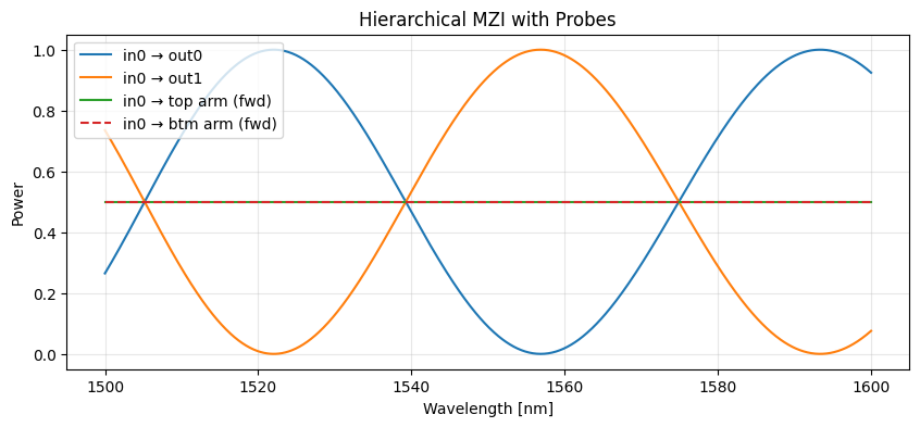
plt.figure(figsize=(10, 4))
plt.plot(wl * 1e3, jnp.abs(S["in0", "out0"]) ** 2, label="in0 → out0")
plt.plot(wl * 1e3, jnp.abs(S["in0", "out1"]) ** 2, label="in0 → out1")
plt.plot(wl * 1e3, jnp.abs(S["in0", "top_arm_fwd"]) ** 2, label="in0 → top arm (fwd)")
plt.plot(wl * 1e3, jnp.abs(S["in0", "btm_arm_fwd"]) ** 2, label="in0 → btm arm (fwd)", ls="--")  # fmt: skip
plt.xlabel("Wavelength [nm]")
plt.ylabel("Power")
plt.title("Hierarchical MZI with Probes")
plt.legend()
plt.ylim(-0.05, 1.05)
plt.grid(True, alpha=0.3)
plt.show()