Quick Start

meow Introduction and Quick Start

Installation

pip install meow-sim

Quick Start

1. Structure

First create the structures to be simulated. A Structure is a collection of a Geometry with a Material.

Note

meow expects the propagation direction to be the z-axis! This makes the zx-plane parallel with the chip and the y-axis perpendicular to the chip. Keep this in mind when creating your structures.

length = 10.0

oxide = mw.Structure(
    material=mw.silicon_oxide,
    geometry=mw.Box(
        x_min=-1.0,
        x_max=1.0,
        y_min=-1.0,
        y_max=0.0,
        z_min=0.0,
        z_max=length,
    ),
)

core = mw.Structure(
    material=mw.silicon,
    geometry=mw.Box(
        x_min=-0.45 / 2,
        x_max=0.45 / 2,
        y_min=0.0,
        y_max=0.22,
        z_min=0,
        z_max=length,
    ),
)

structures = [oxide, core]
mw.visualize(structures)

Note

you can also extrude structures from a gds file. See GdsExtrusionRule.

2. Cells

Once you have a list of Structure objects, they need to be divided into cells. A Cell is a combination of those structures with 2D meshing info (Mesh2d) and a cell length.

num_cells = 5

cells = mw.create_cells(
    structures=structures,
    mesh=mw.Mesh2D(
        x=np.linspace(-1, 1, 101),
        y=np.linspace(-1, 1, 101),
        # specify possible conformal mesh specifications here:
        # bend_radius=2.0,
        # bend_axis=1,
        ez_interfaces=True,
    ),
    Ls=np.array([length / num_cells for _ in range(num_cells)]),
)

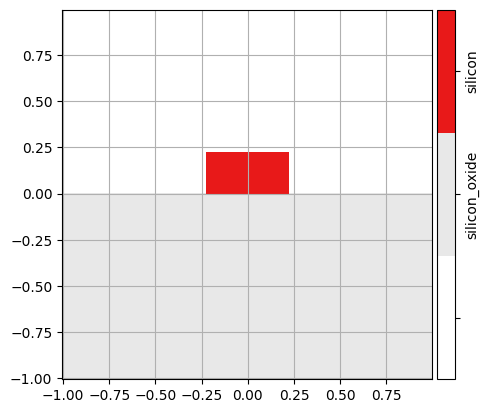
A cell should be a region of (approximate) constant cross section. We can use the visualize() function to show the cross section of a cell:

mw.visualize(cells[0])

3. Cross Sections

A Cell contains all the Structure info, but does not take any Environment information (such as temparature or wavelength) into account. This information is important as it influences the refractive index of the CrossSection.

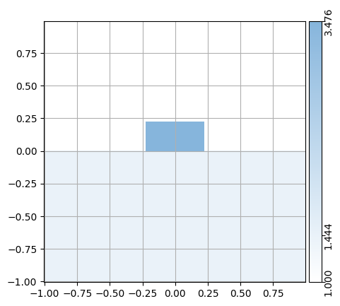
Therefore, combining a Cell with an Environment yields a CrossSection:

env = mw.Environment(wl=1.55, T=25.0)
css = [mw.CrossSection.from_cell(cell=cell, env=env) for cell in cells]
mw.visualize(css[0])

4. Find Modes (FDE)

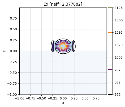
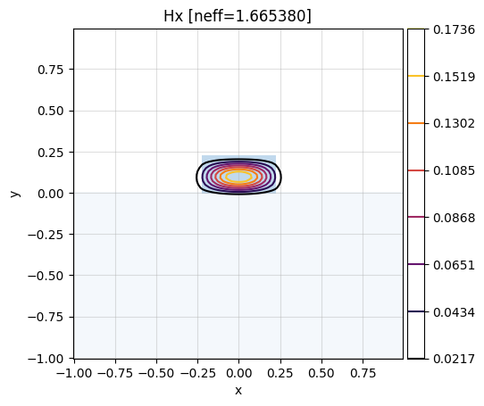
We can now compute multiple Modes per CrossSection using compute_modes():

num_modes = 4

modes: List[List[mw.Mode]] = []
for cs in css:
    modes_in_cs = mw.compute_modes(cs, num_modes=num_modes)
    modes.append(modes_in_cs)

# show Ex component of the first mode (idx 0)
# of the first cell (idx 0):
mw.visualize(modes[0][0], fields=["Ex"])
# show Hx component of the second mode (idx 1)
# of the first cell (idx 0):
mw.visualize(modes[0][1], fields=["Hx"])

Note

above, the Modes of the CrossSection are calculated sequentially. However, you’re invited to try calculating the modes concurrently as well 😉

5. Calculate S-matrix (EME)

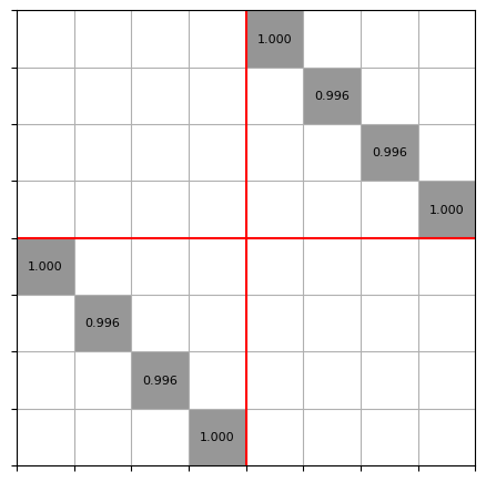
The S-matrix of a collection of modes can now easily be calculated with compute_s_matrix(). This step uses the sax circuit solver under the hood. The resulting S-matrix has is formated such that S[0][0] is the complex reflection coefficient from the fundamental mode into the backwards propagating fundamental mode. S[num_modes][0] is the transmission from the fundamental mode into the fundamental mode, following the pattern S[<to_port>][<from_port>]. The mapping from ports to indices is provided in port_map.

S, port_map = mw.compute_s_matrix(modes, cells)

print(port_map)
mw.visualize((abs(S), port_map))

{'left@0': 0, 'left@1': 1, 'left@2': 2, 'left@3': 3, 'right@0': 4, 'right@1': 5, 'right@2': 6, 'right@3': 7}

That’s it! this was a quick introduction to the meow library!